
Spatial preprocessing#
If you haven’t gone through the temporal_preprocessing.ipynb notebook, please do so first!
In the previous notebook, we’ve looked at how to temporally preprocess our signal through high-pass filtering, prewhitening, and nuisance regression. Importantly, these operations are performed on the timeseries of each voxel separately! Essentially, given our 4D fMRI data (\(X \times Y \times Z \times T\)), temporal filtering as we discussed here is only applied to the fourth dimension (the time-dimension, \(T\)).
In addition to these temporal operations, there are several spatial operations performed on (f)MRI data, including spatial smoothing (a form of filtering), distortion correction, and spatial registration/resampling, which are discussed in this notebook.
What you’ll learn: after this lab, you’ll …
explain the necessity of motion correction and the advantage of motion regression
know how to implement the concepts above in Python
Estimated time needed to complete: 4-6 hours
# import some functionality
import os.path as op
import numpy as np
import nibabel as nib
import matplotlib.pyplot as plt
from scipy.ndimage import gaussian_filter
Spatial filtering (blurring/smoothing)#
Spatial filtering refers to operations applied to the spatial dimensions (\(X\), \(Y\), and \(Z\)) of our 4D data. The most common spatial filtering operation — spatial smoothing — is usually implemented using a “3D gaussian (low-pass) smoothing kernel”. Sounds familiar? Well, it should, because it’s essentially the same type of filter as we used for our temporal high-pass filter! Only this time, it’s not a 1-dimensional gaussian (“kernel”) that does the high-pass filtering, but it’s a 3-dimensional gaussian that does low-pass filtering. Just like the temporal gaussian-weighted running line smoother is applied across time, we apply the 3D gaussian across space (i.e., the 3 spatial dimensions, \(X\), \(Y\), and \(Z\)). The figure below schematically visualized the process*:
(Note that we show the spatial data in 2D, simply because it’s easier to visualize, but in reality this is always 3D!)
In fact, because both (high-pass) temporal filtering and (low-pass) spatial filtering in most fMRI applications depend on the same “gaussian filtering” principle, we can even use the same Python function: gaussian_filter! However, as we mentioned before, spatial smoothing in fMRI is used as a low-pass filter, which means that the (spatial!) frequencies higher than a certain cutoff are filtered out, while the (spatial!) frequencies lower than this cut-off are passed. Therefore, we don’t need to subtract the output from the gaussian_filter function from the (spatial) data! (If we’d would that, than we’re effectively high-pass filtering the data!)
* 3D gaussian figure from Philipp Klaus.
Before we go on and demonstrate smoothing on fMRI data, we need to determine the sigma of our (3D) gaussian kernel that we’ll use to smooth the data. Annoyingly, smoothing kernels in the fMRI literature (and software packages!) are usually not reported in terms of sigma, but as “full-width half maximum” (FWHM), which refers to the width of the gaussian at half the maximum height:
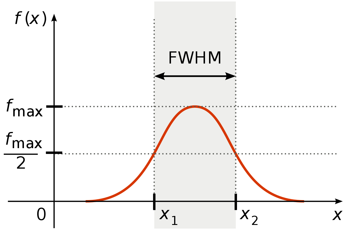
For example, you might read in papers something like “We smoothed our data with a gaussian kernel with a FWHM of 3 millimeter”. So, we need to convert our desired FWHM (in millimeters) to sigma. In fact, this is the same conversion that we needed to do for our temporal Gaussian running line high-pass filter, but this time applied to the spatial domain (i.e., FWHM in mm) instead of the temporal domain (i.e., TR in seconds). We can use the same formula to convert FWHM (in mm.) to sigma:
So, for example, if I want to smooth at FWHM = 6 mm and my voxels are 3 mm in size (assuming equal size in the three spatial dimensions, which is common), my sigma becomes:
The entire conversion process is a bit annoying, but it’s simply necessary due to conventions in the fMRI literature/software packages.
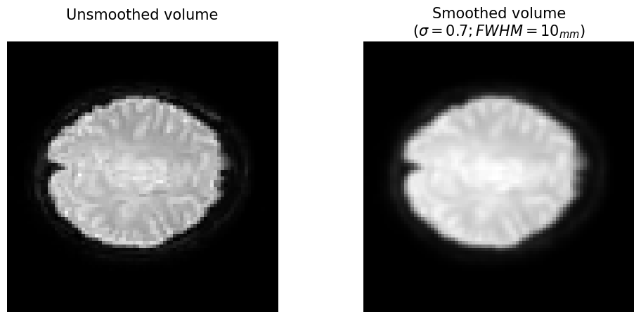
Anyway, having dealt with the conversion issue, let’s look at an example. We’ll use the 4D fMRI data from before (the data_4d variable) and we’ll extract a single 3D volume which we’ll smooth using the gaussian_filter function. This particular data has a voxel-size of \(6\ mm^{3}\); given that we want to smooth at an FWHM of, let’s say, 10 millimeter, we need a sigma of \(\frac{10}{\sqrt{8 \ln{2}} \cdot 6} \approx 0.7\).
f = op.join(op.dirname(op.abspath('')), 'week_1', 'func.nii.gz')
data_4d = nib.load(f).get_fdata()
vol = data_4d[:, :, :, 20] # We'll pick the 21st volume (Python is 0-indexed, remember?)

fwhm = 10
voxelsize = 6

sigma = fwhm / (np.sqrt(8 * np.log(2)) * voxelsize)
smoothed_vol = gaussian_filter(vol, sigma=sigma)

# Let's plot both the unsmoothed and smoothed volume
plt.figure(figsize=(12, 5))
plt.subplot(1, 2, 1)
plt.imshow(vol[:, :, 30], cmap='gray') # And we'll pick the 11th axial slice to visualize
plt.axis('off')
plt.title("Unsmoothed volume\n", fontsize=15)

plt.subplot(1, 2, 2)
plt.imshow(smoothed_vol[:, :, 30], cmap='gray')
plt.axis('off')
plt.title('Smoothed volume\n($\sigma = %.1f; FWHM = %s_{mm}$)' % (sigma, fwhm), fontsize=15)
plt.show()
# Implement your ToDo here

data_4d_smoothed = np.zeros(data_4d.shape)

# YOUR CODE HERE
raise NotImplementedError()
''' Tests the ToDo above '''
from niedu.tests.nii.week_4 import test_smoothing_todo
test_smoothing_todo(data_4d, data_4d_smoothed)
YOUR ANSWER HERE
Susceptibility distortion correction (SDC)#
Most functional MRI sequences use a technique called “gradient-echo echo planar imaging” (GE-EPI), which is a relatively sensitive and well-established technique for BOLD-MRI. For reasons beyond the scope of this course, GE-EPI scans unfortunately show signs of “geometric distortion” (sometimes called susceptibility distortion) and signal loss in some areas of the brain. Signal loss, which is most apparent in areas with B0 (static magnetic field) inhomogeneities caused by sudden air-tissue transitions (like around the ears, earduct → brain, and the ventromedial cortex, frontal sinus → brain). Geometric distortion is most visible in the phase-encoding direction of the scan (usually posterior → anterior or left → right). These geometric distorions are usually visible as tissue “folding” inwards or outwards (depending on the exact phase-encoding direction, e.g., posterior → anterior or anterior → posterior).
In the gif below, you can see where signal loss (in ventromedial cortex and around the ears, best visible in slice z=12) and geometric distortion is most apparent. The “before” image is the one with geometric distortion (most apparent as folding inwards of the cerebellum and frontal cortex). Hover your cursor above the image to see it changing from uncorrected (“before”) to corrected (“after”).
While there is (currently) no way to correct for signal loss, there are ways to correct for geometric distortion (as you can see in the gif above). Most distortion correction techniques require you to acquire additional scans that can be used to correct (or “unwarp”) your functional MRI scans. One technique is to acquire a “fieldmap” scan to image the homogeneity of the magnetic field (based on two scans with slightly different TEs) which can then be used for geometric correction. Another technique, often called “topup unwarping” (or PEPOLAR unwarping), uses one or more volumes of a separate functional MRI scan with the opposite phase-encoding direction as your to-be-correction functional MRI scan. In the “topup” scan, the distortion is expected to be in the complete opposite direction as in your to-be-correction fMRI scan (e.g., inward folding of tissue where the fMRI scan would show outward folding and vice versa), which can then be used to estimate an undistorted shape (which is “in the middle” of the fMRI and topup scan).
The mathematics and implementation of distortion correction is beyond the scope of this course, but we just wanted it to show you so that you’re familiar with the term!
Motion correction / realignment#
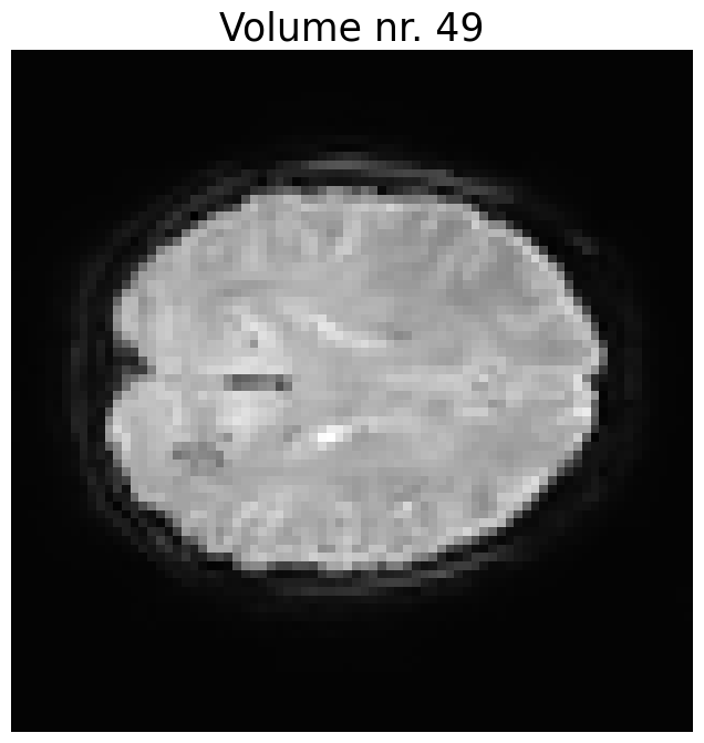
Participant movement during scanning arguably affects your data quality most, and should be taken care of accordingly. As such, motion correction (or sometimes called motion realignment) is an important step in any preprocessing pipeline. Motion correction makes sure that all volumes (i.e., 3D fMRI images) are spatially aligned. Before discussing motion correction in more detail, let’s take a look at how a motion corrupted scan looks like. Actually, the data that we’ve been using so far (data_4d) actually has very little motion, so we’re going to add some motion to it (with a custom function add_motion_to_vols). Then, we’ll plot it volume by volume as a short movie:
from niedu.utils.nii import add_motion_to_vols, animate_volumes

vols = add_motion_to_vols(data_4d)
animate_volumes(vols)
Rigid body registration#
Motion correction aligns all volumes by picking a reference volume (usually the first or middle one) and subsequently “moving” all the other volumes such that they are spatially aligned with the reference volume. Specifically, motion correction uses translation (movement along the primary axes: left/right, up/down, front/back) and rotation (around the center of the image).
 Image from Arcoverde Neto et al. (2014).
This specific transformation of the image has six parameters (translation in the X, Y, and Z direction, and rotation in the X, Y, and Z direction) and is often called a “rigid body registration”. Given these parameters, the to-be-moved volume can be spatially resampled at the location of the reference volume.
A rigid body registration is an example of a more general affine registration: a linear transformation of an image that may involve translation, rotation, scaling, and shearing. For motion correction, scaling and shearing is not applied.
Affine registrations#
For affine registrations, the way the image should be moved is defined in the affine matrix, a \(4 \times 4\) matrix. This matrix is similar to the one we discussed in week 1, but instead of describing how each image coordinate (\(i, j, k\)) relates to world coordinates (\(x, y, z\)), the affine matrix, here, describes how the coordinates from the original (non-corrected) image related to the corrected image:
For example, suppose I have a particular affine matrix (A_example, below) that encodes a translation of 3 voxels downwards (superior → inferior). Then, for any coordinate \((x, y, z, 1)\), I can compute the location of the coordinate in the corrected image as follows:
A_example = np.array([
    [1, 0, 0, 0],
    [0, 1, 0, 0],
    [0, 0, 1, 3],
    [0, 0, 0, 1]
])

# Note that we always have to append a 1, just like in week 1
coord = np.array([0, 0, 0, 1])  # the middle of the image!
corr_coord = A_example @ coord
print(corr_coord[:3])
[0 0 3]
As expected, the affine transformation above shows us that the middle coordinate \((0, 0, 0)\) refers to the corrected coordinate \((0, 0, 3)\) after translating the image 3 voxels downwards. But how is this particular translation encoded in the affine? For translation, this is relatively straightforward. For any translation \((x, y, z)\), the affine matrix looks like:
For rotation, however, it is slightly more complicated! For rotation transformations (with rotations \(x, y, z\) in radians), the affine is computed by the matrix
As you can see, rotations are actually encoded in the affine matrix as the result of matrix multiplication of the the separate x, y, and z rotation matrices. Don’t worry, you don’t have to program this rotation-to-affine operation. Using a custom function (get_rotation_matrix), let’s take a look at what the affine matrix would look like for a rotation of 45 degrees in every direction:
def get_rotation_matrix(x=0, y=0, z=0):
    """ Computes the rotation matrix.

    Parameters
    ----------
    x : float
        Rotation in the x (first) dimension in degrees
    y : float
        Rotation in the y (second) dimension in degrees
    z : float
        Rotation in the z (third) dimension in degrees

    Returns
    -------
    rot_mat : numpy ndarray
        Numpy array of shape 4 x 4
    """

    x = np.deg2rad(x)
    y = np.deg2rad(y)
    z = np.deg2rad(z)

    rot_roll = np.array([
        [1, 0, 0, 0],
        [0, np.cos(x), -np.sin(x), 0],
        [0, np.sin(x), np.cos(x), 0],
        [0, 0, 0, 1]
    ])

    rot_pitch = np.array([
        [np.cos(y), 0, np.sin(y), 0],
        [0, 1, 0, 0],
        [-np.sin(y), 0, np.cos(y), 0],
        [0, 0, 0, 1]
    ])

    rot_yaw = np.array([
        [np.cos(z), -np.sin(z), 0, 0],
        [np.sin(z), np.cos(z), 0, 0],
        [0, 0, 1, 0],
        [0, 0, 0, 1]
    ])

    rot_mat = rot_roll @ rot_pitch @ rot_yaw
    return rot_mat


A_rot = get_rotation_matrix(x=45, y=45, z=45)
print(A_rot)
[[ 0.5        -0.5         0.70710678  0.        ]
 [ 0.85355339  0.14644661 -0.5         0.        ]
 [ 0.14644661  0.85355339  0.5         0.        ]
 [ 0.          0.          0.          1.        ]]
Now, if we want to combine both rotations and translations, we multiply the translation matrix (\(T\)) with our rotation matrix (\(R = R_{x}R_{y}R_{z}\)):
def get_translation_matrix(x=0, y=0, z=0):
    """ Computes the translation matrix.

    Parameters
    ----------
    x : float
        Translation in the x (first) dimension in voxels
    y : float
        Rotation in the y (second) dimension in voxels
    z : float
        Rotation in the z (third) dimension in voxels

    Returns
    -------
    trans_mat : numpy ndarray
        Numpy array of shape 4 x 4
    """

    trans_mat = np.eye(4)
    trans_mat[:, -1] = [x, y, z, 1]
    return trans_mat

# YOUR CODE HERE
raise NotImplementedError()
''' Tests the above ToDo. '''
from niedu.tests.nii.week_4 import test_affine_todo
test_affine_todo(affine_todo)
Now, we’re not going to discuss the intricacies of how to actually resample an image given a particular affine. Instead, we defined a function called resample_image that resamples an image given a particular translation and rotation matrix. It’s a bit more complicated than we discussed so far, but you get the idea.
from scipy.ndimage import affine_transform

def resample_image(image, trans_mat, rot_mat):
    """ Resamples an image given a translation and rotation matrix.

    Parameters
    ----------
    image : numpy array
        A 3D numpy array with image data
    trans_mat : numpy array
        A numpy array of shape 4 x 4
    rot_mat : numpy array
        A numpy array of shape 4 x 4

    Returns
    -------
    image_reg : numpy array
        A transformed 3D numpy array
    """

    # We need to rotate around the origin, not (0, 0), so
    # add a "center" translation
    center = np.eye(4)
    center[:3, -1] = np.array(image.shape) // 2 - 0.5
    A = center @ trans_mat @ rot_mat @ np.linalg.inv(center)

    # affine_transform does "pull" resampling by default, so
    # we need the inverse of A
    image_corr = affine_transform(image, matrix=np.linalg.inv(A))

    return image_corr
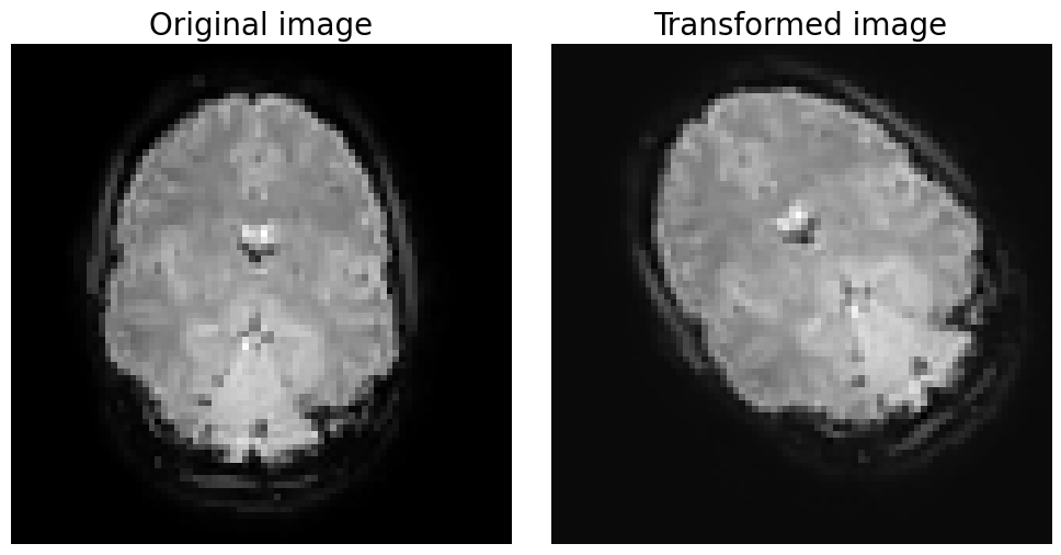
trans_mat = get_translation_matrix(5, 5, 0)
rot_mat = get_rotation_matrix(0, 0, 40)

vols = data_4d
VOL = vols[:, :, :, 0]
PLOT_AXIS = 2
SLICE_IDX = 20

plt.figure(figsize=(10, 5))
plt.subplot(1, 2, 1)
plt.imshow(np.take(VOL, SLICE_IDX, PLOT_AXIS).T, origin='lower', cmap='gray')
plt.axis('off')
plt.title('Original image', fontsize=20)

# Resample
vol_res = resample_image(VOL, trans_mat, rot_mat)

plt.subplot(1, 2, 2)
plt.imshow(np.take(vol_res, SLICE_IDX, PLOT_AXIS).T, origin='lower', cmap='gray')
plt.axis('off')
plt.title('Transformed image', fontsize=20)

plt.tight_layout()
plt.show()
Now, suppose that we want to align two volumes with each other. How would we go about it? Visually, it’s quite hard to assess whether a particular affine matrix works well. In practice, most neuroimaging software packages use automatic algorithms that try to find a affine matrix that minimizes some cost function. In other words, it defines a function to evaluate the mismatch (or cost) of the alignment of two volumes given an affine matrix, and then it tries to minimize this function by (in a smart way) trying out different rotation and translation parameters.
One cost function that is often used for rigid body registration is “least squares”, which is defined as the sum over the squared (voxel-wise, \(v\)) differences between the reference image (sometimes called the “fixed” image) and the realigned image (sometimes called the “moving” image):
# YOUR CODE HERE
raise NotImplementedError()
""" Tests the above ToDo """
fixed = np.ones((10, 10, 10))
moving = np.zeros((10, 10, 10))

np.testing.assert_almost_equal(least_squares_cost(fixed, moving), 1000)

fixed = np.arange(1000).reshape((10, 10, 10))
moving = fixed[::-1]
np.testing.assert_almost_equal(least_squares_cost(fixed, moving), 330000000)

moving = np.roll(fixed.ravel(), 1).reshape((10, 10, 10))
np.testing.assert_almost_equal(least_squares_cost(fixed, moving), 999000)

print("Well done!")
Hint 1: you need rotation in the z dimension and translation in the x and y dimension.
Hint 2: rotation is counter clockwise (if you define negative rotation, e.g. -20, it will be rotated clockwise).
with np.load('moco_todo.npz') as moco_data:
    moving = moco_data['moving']
    fixed = moco_data['fixed']

# YOUR CODE HERE
raise NotImplementedError()

### Plotting starts here
# Only works if you've defined a variable named 'moved'
# Do not change the code below
plt.figure(figsize=(10, 10))
plt.imshow(fixed[:, :, 25].T, origin='lower', cmap='gray')
moved4plot = np.ma.masked_where(moved < 2, moved)
plt.imshow(moved4plot[:, :, 25].T, origin='lower', alpha=0.8)
plt.axis('off')
plt.show()
Anatomical realignment/registration and normalization#
So far, we discussed how to register volumes to a reference volume using rigid body registrations (with a six parameter affine) in the context of motion correction. This is, however, only the first step in the complete registration protocol of (most) studies. If your goal is, in the end, to perform some kind of group analysis (in which you pool together data from multiple subjects), you want to make sure that each voxel (at location \((X, Y, Z)\)) is in (roughly) the same location in the brain. The problem is that people’s brains differ quite a bit in terms of anatomy! Therefore, you need to register (transform) your subject-level (functional) data to some kind of common template. This process is often done in two stages: first, you compute a registration from (a reference volume of) your functional data (“moving”) to your anatomical data (your high-resolution T1-weighted scan; “fixed”), and second you compute a registration from your anatomical data (“moving”) to a common template (“fixed”). Then, you can register your functional data to the common template by sequentially applying the first and second stage registration parameters. This is visualized in the figure below.
In the figure above, you can see that the first stage (BOLD → T1w) uses the same registration protocol as we used with motion-correction: an affine transformation with 6 parameters (translation and rotation in 3 directions; a “rigid body registration”). The second stage (T1w → template) also uses an affine transformation, but this time with 12 parameters. In addition to the 6 rigid body registration parameters, a 12 parameter affine (sometimes reffered to as an affine with 12 degrees-of-freedom, DOF) also includes global scaling in 3 directions (i.e., making the brain bigger of smaller) and shearing in 3 directions (i.e., “stretching” in 3 directions). These extra parameters attempt to overcome the anatomical differences between the individual subjects’ brains and the template.
However, only a 12 DOF affine is usually not sufficient for proper alignment. Therfore, most neuroimaging software packages also offer the option to apply a non-linear registration step (“warping”) on top of the 12 DOF affine registration. Instead of globally transforming your “moving” volume (i.e., the transformation applies to each voxel equally), non-linear registrations allow for local transformations (i.e., some voxels might be transformed “more” than others). Usually, the combination of an initial 12 DOF affine and a non-linear (“warping”) registration operation lead to a proper alignment of the subject’s anatomical volume and the template.
YOUR ANSWER HERE
Motion filtering#
Even after motion realignment, your data is still ‘contaminated’ by motion. This is because movement itself influences the measured activity. For example, suppose that you measure a single voxel in someone’s brain; then, this person moves his/her head 2 centimeters. Now, we can do motion realigment to make sure we measure the same voxel before and after the movement, but this does not change the fact that this particular voxel was originally measured at two different locations. It could be that after the movement, the voxel was actually a little bit closer to the headcoil, which results in a (slight) increase in signal compared to before the movement (this is also known as “spin history effects”).
Ideally, you want to account for these interactions between motion and the measured activity. One way to do this is through “motion filtering”, of which one popular approach is to simply add the 6 realignment parameters (rotation and translation in 3 directions) to the design-matrix (\(X\))! In other words, we treat the motion realignment parameters as “nuisance regressors” that are aimed to explain activity that is related to motion. Realize that this is, thus, as temporal preprocessing step (which we discuss here instead of the previous notebook because we needed to explain motion correction first).
Alright, let’s load some realigment parameters (6 in total) from an fMRI run of 200 volumes. We’ll plot them below:
""" This data has been motion-corrected using the FSL tool 'MCFLIRT', which outputs a file
ending in *.par that contains the 6 motion parameters (rotation/translation in 3 directions each).
We'll load in this file and plot these motion parameters. """

motion_params = np.loadtxt('func_motion_pars_new.txt')
rotation_params = motion_params[:, :3]
translation_params = motion_params[:, 3:]

plt.figure(figsize=(15, 7))
plt.subplot(2, 1, 1)
plt.title('Rotation', fontsize=25)
plt.plot(rotation_params)
plt.xlim(0, motion_params.shape[0])
plt.legend(['x', 'y', 'z'], fontsize=15)
plt.ylabel('Rotation in radians', fontsize=15)
plt.grid()

plt.subplot(2, 1, 2)
plt.title('Translation', fontsize=25)
plt.plot(translation_params)
plt.legend(['x', 'y', 'z'], fontsize=15)
plt.ylabel('Translation in mm', fontsize=15)
plt.xlim(0, motion_params.shape[0])
plt.xlabel('Time (TR)', fontsize=15)
plt.grid()

plt.tight_layout()
plt.show()
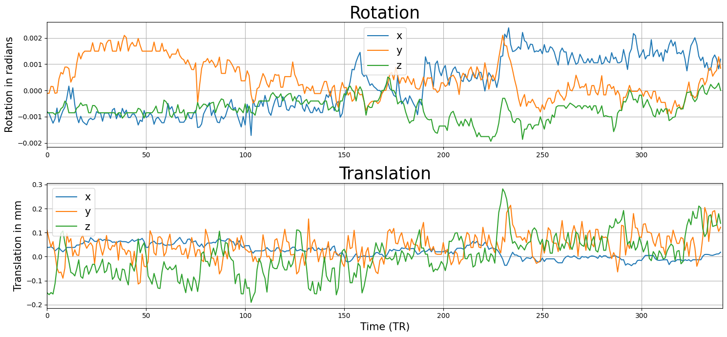
So, is this good data or not? In general, you could say that higher values (in either translation or rotation) are worse. That said, from the translation and rotation parameters alone it is hard to judge whether the participant moved too much, partly because we’re dealing with 6 parameter traces here. One way to make this decision process a little easier is to convert these parameters to a single “framewise displacement” (FD) trace. FD aims to represent “bulk motion” and is a summary statistic of motion that combines all motion parameters into a single metric. It is calculated as follows:
where \(|x|\) means the absolute value of \(x\) and \(r\) stands for a predefined radius in millimeters (which is usually taken to be 50). So, basically it is a sum across the absolute successive differences (\(x_{t} - x_{t-1}\)) of parameter traces.
# Implement the optional ToDo here
# YOUR CODE HERE
raise NotImplementedError()
''' Tests the above ToDo. '''
from niedu.tests.nii.week_4 import test_fd_calc
test_fd_calc(motion_params, fd_trace)
As said in the beginning of this section, motion parameters (translation/rotation in 3 dimensions) are used as nuisance regressors in subject-level analyses. The reason for this is that, even after motion correction, the actual movement may have influenced the signal intensity through “spin-history effects”, which occurs when a voxel is excited by an RF pulse slightly earlier/later due to movement (i.e., it may have moved up or down one slice), which changes how much T1 relaxation occurs (which affect the signal intensity; read more here).
There are two ways to go about this, which are not mutually exclusive. The most common way (in task-based fMRI) is to add the six motion parameters (rotation/translation in three directions) to your design. Any variance of your signal that covaries with (one or more of) these motion parameters will be accounted for (and will thus not end up in your noise term).
# Implement your ToDo here
# YOUR CODE HERE
raise NotImplementedError()
''' Tests the above ToDo. '''
from niedu.tests.nii.week_4 import test_friston24
test_friston24(motion_params, friston24)
Apart from directly adding the (extended) motion parameters to your design, you can also perform “motion scrubbing”. Motion scrubbing is usually performed in resting-state analyses and is conceptually very similar to the “despiking” we did earlier. With motion scrubbing, you usually set a predefined threshold for your FD trace (for example 1 mm) and any timepoint above this threshold will be “scrubbed out”. This is done by defining a separate regressor for each timepoint above the threshold containing all zeros except for the above-threshold timepoint, which contains a zero (just like we did with despiking). Sometimes, even the timepoint before and/or after the “bad” timepoint are additionally added to the design matrix. As this course focuses mostly on task-based fMRI analyses, we won’t discuss motion scrubbing any further (but if you want to know more about the different motion correction strategies, we recommend the following article: Power et al., 2015).
For this ToDo, you have to compare two models and the resulting (normalized) effects (t-values): a model without the six motion parameters and a model with the six motion parameters. You should use the motion_params variable which we defined earlier as your motion parameters.
We provide you with a design-matrix (X) with an intercept and a single stimulus-predictor and the signal of a single voxel (sig). Calculate the t-value for the contrast of the predictor-of-interest against baseline for both the original design-matrix (only intercept + predictor-of-interest; store this in a variable named tval_simple) and the design-matrix extended with the six motion parameters (which thus has 8 predictors; store this in a variable named tval_ext).
# First, we'll load the data
with np.load('data_motion_filtering.npz') as data_last_todo:
    X = data_last_todo['X']
    sig = data_last_todo['sig']

print("Shape of original X: %s" % (X.shape,))
print("Shape of signal: %s" % (sig.shape,))
Shape of original X: (341, 2)
Shape of signal: (341,)
""" Implement the ToDo here. """

# YOUR CODE HERE
raise NotImplementedError()
''' Tests the above ToDo. '''
from niedu.tests.nii.week_4 import test_tvals_motion
test_tvals_motion(X, sig, motion_params, tval_simple, tval_ext)
YOUR ANSWER HERE
Alright, that’s it for preprocessing! If you want to know more about a preprocessing software package that we particularly like, check out the next (optional) notebook about Fmriprep (fmriprep.ipynb)!