
First-level analyses (using FSL)#
This notebook provides the first part (first-level analysis) of an introduction to multilevel models and how to implement them in FSL. The next notebook, run_level_analysis.ipynb, will continue with run-level analysis, and next week we will conclude this topic with group-level analyses. If you haven’t done so already, please go throught linux_and_the_command_line notebook first!
You actually know most about “first-level analyses” already, as it describes the process of modelling single-subject (single-run) timeseries data using the GLM, which we discussed at length in week 2. In this notebook, you’ll learn how to use FSL for (preprocessing and) first-level analyses. Note that there are several other excellent neuroimaging software packages, such as SPM (Matlab-based), AFNI, BROCCOLI, Freesurfer, and Nilearn. In fact, in week 7, there is a notebook on how to use Nilearn to fit statistical models on fMRI data.
We like FSL in particular, as it’s a mature and well-maintained package, free and open-source, and provides both a graphical interface and a command line interface for most of its tools.
What you’ll learn: after this lab, you’ll be able to …
visualize and inspect (f)MRI in FSLeyes;
set up a first-level model in FSL FEAT
Estimated time needed to complete: 2-4 hours
# Import functionality
import numpy as np
import matplotlib.pyplot as plt
%matplotlib inline
Using FSLeyes#
In the previous notebook about Linux and the command line, we discussed how to use built-in Linux commands and FSL-specific commands using the command line. Now, let’s focus on using a specific FSL tool called “FSLeyes”, which is a useful program to view (f)MRI files (basically any nifti-file). We can start this graphical tool from the command line with the command: fsleyes &. We append the & to the FSLeyes command because this makes sure FSLeyes will run “in the background” and thus allows us to keep using the command line (if we would not use the &, FSLeyes would run be active “in your terminal”, and we wouldn’t be able to use that anymore).
This should open a new window with FSLeyes. Now, let’s open a file!
Now, FSLeyes should look similar to the figure below.

As you can see, FSLeyes consists of multiple views, panels, and toolbars. You should see an anatomical MRI image shown in three perspectives (sagittal, coronal, and axial) with green crosshairs in the “Ortho view”.
Notice the labels on the sides of the image: P (posterior), A (anterior), I (inferior), S (superior), L (left), and R (right).
In the “Overlay toolbar”, you can adjust both the brightness and contrast of the image. One could argue that the default settings are a little bit too dark (for this scan at least).
Importantly, while moving the location of the crosshairs, you see in the lower right corner (under the “Location panel”) that some numbers change. The left side of the panel shows you both the location of the crosshairs in “world coordinates” (relative to the isocenter of the scanner, in millimeters) and in “voxel coordinates” (starting from 0).
The right side of the panel shows you the voxel coordinates of the crosshairs together with the signal intensity, e.g., \([156\ 123\ 87]: 600774.75\). Try changing the crosshairs from a voxel in the CSF, to a voxel in gray matter, and a voxel in white matter and observe how the signal intensity changes.
# Replace the Nones with the correct numbers
X = None
Y = None
Z = None

# YOUR CODE HERE
raise NotImplementedError()
''' Tests the above ToDo.'''
from niedu.tests.nii.week_5 import test_how_many_slices_fsleyes
test_how_many_slices_fsleyes(X, Y, Z)
Now, let’s check out some functional data (fMRI) in FSLeyes!
FSLeyes neatly plots the functional data on top of the anatomical image. Note that the resolution differs between the anatomical (\(1 \times 1 \times 1\) mm) and functional (\(2.7 \times 2.7 \times 2.97\) mm)! FSLeyes still allows you to view these images on top of each other by interpolating the images.
Now, let’s make our view a little bit nicer.
Setting a minimum value will threshold the image at this value, which will mask most of the background. Now, let’s also change the color scheme for the func file to be able to distinguish the func and anat file a little better:
Now you can clearly see that setting a threshold did not mask all non-brain tissue, as some skull seems to still show “activity”!
Again, just like with the anatomical scan, the “Location panel” shows you both the (voxel and world) coordinates as well as the signal intensity.
Instead of manually adjusting the volume number, you can press the “Video” icon (next to the big “+” icon, which you can use to toggle the crosshairs on or off) to start “Movie mode” in which FSLeyes will loop through all volumes. Due to the lag on the server (or a software bug in FSLeyes, I’m not sure), however, FSLeyes is not fast enough to render the volumes, so you’ll likely see a black screen…
That said, looping through your volumes is usually a great way to visually check for artifacts (e.g. spikes) and (extreme) motion in your data! We highly recommend doing this for all your data!
Another useful way to view your fMRI data is using the “Time series” view.
FSLeyes has many more features than we discussed in this section (e.g., working with standard atlases/parcellations). We’ll demontrate these features throughout the rest of this lab where appropriate!
Skullstripping#
When viewing the anatomical scan in the previous section, you might have noticed that the scan still contained the subject’s skull. Usually, the skull is removed because it improves registration to the subject’s anatomical T1-scan (especially if you use BBR-based registration). This process is often called “skullstripping” and FSL contains the skullstripping-tool bet (which stands for “Brain Extraction Tool”). We’ll demonstrate how to use bet using its command-line interface.
Like all FSL tools with command-line interfaces, you can get more info on how to use it by calling the command with the flag --help.
You see that the “bet” command should be called as follows:
bet <input> <output> [options/flags]
We recommend visually checking the result of skullstripping for imperfections (e.g. part of the brain that are excluded or parts of non-brain that are included). Let’s do this in FSLeyes!
Then, load the non-skullstripped anatomical file (sub-02_desc-preproc_T1w.nii.gz) first. Then, overlay the skullstripped image (the sub-02_desc-preproc+bet_T1w.nii.gz file you just created). The difference between the non-skullstripped and the skullstriped image is, now, however not clear; to make this clearer, we can pick a different colormap for the skullstripped brain! For example, change the “Grayscale” colormap to “Red-Yellow”. Also, change the opacity to about 50% to better see the underlying non-skullstripped anatomical scan.
Scroll through the image to see whether bet did a good job.
Also, it failed to remove some non-brain tissue. For example, what non-brain structure do you think is located at \([X=143, Y=178, Z=72]\)? And at \([X=140, Y=124, Z=44]\)?
You could, of course, just skullstrip all your participants without looking at the resulting skullstripped brain images. However, as we just saw, this may lead to suboptimal results, which may bias subsequent preprocessing steps, such as functional → anatomical registration and spatial normalization to a standard template. As such, we recommend visually inspecting the skullstrip result for each participant in your dataset!
If you find that bet did not do a proper job, you can adjust several parameters to improve the skullstripping operation. The two most useful parameters to adjust are “robust brain centre estimation” (flag -R), “fractional intensity threshold” (flag -f <value>), and the vertical gradient (flag -g <values>). We recommend always enabling “robust brain centre estimation” (which iterates the operation multiple times, which usually gives more robust results).
The proper value for fractional intensity threshold (-f) and the vertical gradient (-g), however, you need to “tune” yourself (although the default, 0.5, is a good starting value). Smaller values for fractional intensity threshold give you larger brain outline estimates (i.e., “threshold” to be used for image is lower). With the vertical gradient you can tell bet to be relatively more “aggressive” (with values < 0) or “lenient” (with values > 0) with removing tissue at the bottom (inferior side) of the brain. So, e.g., using -g -0.1 will remove relatively more tissue at the bottom of the brain.
To include these parameters, you can call bet with, for example, a “fractional intensity threshold” of 0.4, a vertical gradient of -0.1, and robust brain centre estimation enabled as follows:
bet <input> <output> -f 0.4 -g -0.1 -R
For this ToDo, try out some different parameters for fractional intensity threshold and vertical gradient, and enable robust brain centre estimation. Note that the output file will be overwritten if you use the same output-name (which is fine if you don’t want to save the previous result). Also, there may not be a combination of settings that creates a “perfect” skullstrip result (at least for this brain).
Once you’re happy with the segmentation, overlay it on the original anatomical file in FSLeyes (and use a different colormap). Then, make a snapshot using the camera icon and save it in your week_5 directory (name it “my_skullstripped_image.png”). After you created and saved the snapshot, add the following line to the answer-cell below:

After adding this to the text-cell below and running the cell, the snapshot should be visible in the notebook. (This allows us to check whether you actually did the ToDo; there is not necessarily a “correct” answer to this ToDo — we just want you to mess around with bet and the command line).
YOUR ANSWER HERE
Note that adjusting the parameters of bet may in fact not completely solve all the imperfections in the skullstripping procedure. If you really care about accurate segmentation (e.g., when doing anatomical analyses such as voxel-based morphometry or surface-based analyses), you may consider editing your skullstrip result manually. FSLeyes has an “edit mode” (Tools → Edit mode) in which can manually fill or erase voxels based on your own judgment what is actual brain tissue and what is not.
Skullstripping is actually the only preprocessing operation you have to do manually using the command line (which might be a good idea, anyway, as you should inspect the result manually). The rest of the preprocessing steps within FSL are actually neatly integrated in the FSL tool “FEAT” (FMRI Expert Analysis Tool), which is FSL’s main analysis workhorse (implementing first-level and grouplevel analyses). We’ll discuss doing first-level and fixed-effect analyses with FEAT later in this tutorial, but first let’s talk about the dataset that we’ll use for the upcoming lab!
The “NI-edu” dataset#
So far in this course, we have used primarily simulated data. From this week onwards, we’ll also use some real data from a dataset (which we’ll call “NI-edu”) acquired at our 3T scanner at the University of Amsterdam. The NI-edu study has been specifically “designed” for this (and the follow-up “pattern analysis”) course. The experimental paradigms used for this dataset are meant to investigate how the brain processes information from faces and the representation of their subjective impressions (e.g., their perceived attractiveness, dominance, and trustworthiness). In addition to tasks that investigate face processing specifically, the dataset also includes several runs with a “functional localizer” task, which can be used to identify regions that preferentially respond to a particular object category (like faces, bodies, characters, etc.). In this course, we’ll mostly use the localizer data, because the associated task (design) is relativelly simple and generates a robust signal.
Below, we download the data needed for this tutorial, which is the anatomical data and functional data from a single run of the flocBLOCKED task (see below) from a single subject (sub-03). The data will be saved in your home directory in a folder named “NI-edu-data”.
import os
data_dir = os.path.join(os.path.expanduser("~"), 'NI-edu-data')
print("Data (+- 110MB) will be saved in %s ..." % data_dir)
print("Go get some coffee. This may take a while.\n")

# Using the CLI interface of the `awscli` Python package, we'll download the data
# Note that we only download the preprocessed data from a single run from a single subject
# This may take about 2-10 minutes or so (depending on your download speed)

# Download anatomical files
!aws s3 sync --no-sign-request s3://openneuro.org/ds003965 {data_dir} --exclude "*" --include "sub-03/ses-1/anat/*"

# And functional files
!aws s3 sync --no-sign-request s3://openneuro.org/ds003965 {data_dir} --exclude "*" --include "sub-03/ses-1/func/*task-flocBLOCKED*"

# And a brain mask (needed for FEAT, later)
!aws s3 sync --no-sign-request s3://openneuro.org/ds003965 {data_dir} --exclude "*" --include "derivatives/fmriprep/sub-03/ses-1/anat/sub-03_ses-1_acq-AxialNsig2Mm1_desc-brain_mask.nii.gz"

print("\nDone!")
Data (+- 110MB) will be saved in /home/runner/NI-edu-data ...
Go get some coffee. This may take a while.
Completed 256.0 KiB/8.3 MiB (799.5 KiB/s) with 2 file(s) remaining
Completed 512.0 KiB/8.3 MiB (1.6 MiB/s) with 2 file(s) remaining
Completed 768.0 KiB/8.3 MiB (2.3 MiB/s) with 2 file(s) remaining
Completed 1.0 MiB/8.3 MiB (3.1 MiB/s) with 2 file(s) remaining
Completed 1.2 MiB/8.3 MiB (3.8 MiB/s) with 2 file(s) remaining
Completed 1.5 MiB/8.3 MiB (4.5 MiB/s) with 2 file(s) remaining
Completed 1.8 MiB/8.3 MiB (5.3 MiB/s) with 2 file(s) remaining
Completed 2.0 MiB/8.3 MiB (6.0 MiB/s) with 2 file(s) remaining
Completed 2.2 MiB/8.3 MiB (6.7 MiB/s) with 2 file(s) remaining
Completed 2.5 MiB/8.3 MiB (7.4 MiB/s) with 2 file(s) remaining
Completed 2.8 MiB/8.3 MiB (8.1 MiB/s) with 2 file(s) remaining
Completed 2.8 MiB/8.3 MiB (8.2 MiB/s) with 2 file(s) remaining
Completed 3.0 MiB/8.3 MiB (8.9 MiB/s) with 2 file(s) remaining
Completed 3.3 MiB/8.3 MiB (9.6 MiB/s) with 2 file(s) remaining
Completed 3.5 MiB/8.3 MiB (10.3 MiB/s) with 2 file(s) remaining
Completed 3.8 MiB/8.3 MiB (11.0 MiB/s) with 2 file(s) remaining
Completed 4.0 MiB/8.3 MiB (11.6 MiB/s) with 2 file(s) remaining
Completed 4.3 MiB/8.3 MiB (12.3 MiB/s) with 2 file(s) remaining
Completed 4.5 MiB/8.3 MiB (13.0 MiB/s) with 2 file(s) remaining
Completed 4.8 MiB/8.3 MiB (13.7 MiB/s) with 2 file(s) remaining
Completed 5.0 MiB/8.3 MiB (14.4 MiB/s) with 2 file(s) remaining
Completed 5.3 MiB/8.3 MiB (15.0 MiB/s) with 2 file(s) remaining
Completed 5.5 MiB/8.3 MiB (15.7 MiB/s) with 2 file(s) remaining
Completed 5.8 MiB/8.3 MiB (16.3 MiB/s) with 2 file(s) remaining
Completed 5.8 MiB/8.3 MiB (16.2 MiB/s) with 2 file(s) remaining
download: s3://openneuro.org/ds003965/sub-03/ses-1/anat/sub-03_ses-1_acq-AxialNsig2Mm1_T1w.json to ../../../../../../NI-edu-data/sub-03/ses-1/anat/sub-03_ses-1_acq-AxialNsig2Mm1_T1w.json
Completed 5.8 MiB/8.3 MiB (16.2 MiB/s) with 1 file(s) remaining
Completed 6.0 MiB/8.3 MiB (16.9 MiB/s) with 1 file(s) remaining
Completed 6.3 MiB/8.3 MiB (17.5 MiB/s) with 1 file(s) remaining
Completed 6.5 MiB/8.3 MiB (18.2 MiB/s) with 1 file(s) remaining
Completed 6.8 MiB/8.3 MiB (18.8 MiB/s) with 1 file(s) remaining
Completed 7.0 MiB/8.3 MiB (19.5 MiB/s) with 1 file(s) remaining
Completed 7.3 MiB/8.3 MiB (20.1 MiB/s) with 1 file(s) remaining
Completed 7.5 MiB/8.3 MiB (20.7 MiB/s) with 1 file(s) remaining
Completed 7.8 MiB/8.3 MiB (21.4 MiB/s) with 1 file(s) remaining
Completed 8.0 MiB/8.3 MiB (22.0 MiB/s) with 1 file(s) remaining
Completed 8.3 MiB/8.3 MiB (22.6 MiB/s) with 1 file(s) remaining
download: s3://openneuro.org/ds003965/sub-03/ses-1/anat/sub-03_ses-1_acq-AxialNsig2Mm1_T1w.nii.gz to ../../../../../../NI-edu-data/sub-03/ses-1/anat/sub-03_ses-1_acq-AxialNsig2Mm1_T1w.nii.gz
Completed 256.0 KiB/114.2 MiB (427.4 KiB/s) with 6 file(s) remaining
Completed 512.0 KiB/114.2 MiB (851.0 KiB/s) with 6 file(s) remaining
Completed 768.0 KiB/114.2 MiB (1.2 MiB/s) with 6 file(s) remaining
Completed 1.0 MiB/114.2 MiB (1.4 MiB/s) with 6 file(s) remaining
Completed 1.2 MiB/114.2 MiB (1.8 MiB/s) with 6 file(s) remaining
Completed 1.5 MiB/114.2 MiB (2.1 MiB/s) with 6 file(s) remaining
Completed 1.8 MiB/114.2 MiB (2.5 MiB/s) with 6 file(s) remaining
Completed 2.0 MiB/114.2 MiB (2.8 MiB/s) with 6 file(s) remaining
Completed 2.2 MiB/114.2 MiB (3.2 MiB/s) with 6 file(s) remaining
Completed 2.5 MiB/114.2 MiB (3.5 MiB/s) with 6 file(s) remaining
Completed 2.8 MiB/114.2 MiB (3.9 MiB/s) with 6 file(s) remaining
Completed 3.0 MiB/114.2 MiB (4.2 MiB/s) with 6 file(s) remaining
Completed 3.2 MiB/114.2 MiB (4.5 MiB/s) with 6 file(s) remaining
Completed 3.5 MiB/114.2 MiB (4.9 MiB/s) with 6 file(s) remaining
Completed 3.8 MiB/114.2 MiB (5.2 MiB/s) with 6 file(s) remaining
Completed 4.0 MiB/114.2 MiB (5.5 MiB/s) with 6 file(s) remaining
Completed 4.2 MiB/114.2 MiB (5.8 MiB/s) with 6 file(s) remaining
Completed 4.5 MiB/114.2 MiB (6.1 MiB/s) with 6 file(s) remaining
Completed 4.8 MiB/114.2 MiB (6.5 MiB/s) with 6 file(s) remaining
Completed 5.0 MiB/114.2 MiB (6.8 MiB/s) with 6 file(s) remaining
Completed 5.2 MiB/114.2 MiB (7.1 MiB/s) with 6 file(s) remaining
Completed 5.5 MiB/114.2 MiB (7.5 MiB/s) with 6 file(s) remaining
Completed 5.8 MiB/114.2 MiB (7.8 MiB/s) with 6 file(s) remaining
Completed 6.0 MiB/114.2 MiB (8.1 MiB/s) with 6 file(s) remaining
Completed 6.2 MiB/114.2 MiB (8.4 MiB/s) with 6 file(s) remaining
Completed 6.5 MiB/114.2 MiB (8.7 MiB/s) with 6 file(s) remaining
Completed 6.8 MiB/114.2 MiB (9.0 MiB/s) with 6 file(s) remaining
Completed 7.0 MiB/114.2 MiB (9.3 MiB/s) with 6 file(s) remaining
Completed 7.2 MiB/114.2 MiB (9.7 MiB/s) with 6 file(s) remaining
Completed 7.5 MiB/114.2 MiB (10.0 MiB/s) with 6 file(s) remaining
Completed 7.8 MiB/114.2 MiB (10.3 MiB/s) with 6 file(s) remaining
Completed 8.0 MiB/114.2 MiB (10.6 MiB/s) with 6 file(s) remaining
Completed 8.2 MiB/114.2 MiB (10.9 MiB/s) with 6 file(s) remaining
Completed 8.5 MiB/114.2 MiB (11.3 MiB/s) with 6 file(s) remaining
Completed 8.8 MiB/114.2 MiB (11.6 MiB/s) with 6 file(s) remaining
Completed 9.0 MiB/114.2 MiB (11.9 MiB/s) with 6 file(s) remaining
Completed 9.2 MiB/114.2 MiB (12.2 MiB/s) with 6 file(s) remaining
Completed 9.5 MiB/114.2 MiB (12.5 MiB/s) with 6 file(s) remaining
Completed 9.8 MiB/114.2 MiB (12.8 MiB/s) with 6 file(s) remaining
Completed 10.0 MiB/114.2 MiB (13.1 MiB/s) with 6 file(s) remaining
Completed 10.2 MiB/114.2 MiB (13.4 MiB/s) with 6 file(s) remaining
Completed 10.5 MiB/114.2 MiB (13.8 MiB/s) with 6 file(s) remaining
Completed 10.8 MiB/114.2 MiB (14.1 MiB/s) with 6 file(s) remaining
Completed 11.0 MiB/114.2 MiB (14.3 MiB/s) with 6 file(s) remaining
Completed 11.2 MiB/114.2 MiB (14.6 MiB/s) with 6 file(s) remaining
Completed 11.5 MiB/114.2 MiB (15.0 MiB/s) with 6 file(s) remaining
Completed 11.8 MiB/114.2 MiB (15.3 MiB/s) with 6 file(s) remaining
Completed 12.0 MiB/114.2 MiB (15.5 MiB/s) with 6 file(s) remaining
Completed 12.2 MiB/114.2 MiB (15.8 MiB/s) with 6 file(s) remaining
Completed 12.5 MiB/114.2 MiB (16.0 MiB/s) with 6 file(s) remaining
Completed 12.8 MiB/114.2 MiB (16.3 MiB/s) with 6 file(s) remaining
Completed 13.0 MiB/114.2 MiB (16.6 MiB/s) with 6 file(s) remaining
Completed 13.2 MiB/114.2 MiB (16.8 MiB/s) with 6 file(s) remaining
Completed 13.5 MiB/114.2 MiB (17.2 MiB/s) with 6 file(s) remaining
Completed 13.8 MiB/114.2 MiB (17.5 MiB/s) with 6 file(s) remaining
Completed 14.0 MiB/114.2 MiB (17.8 MiB/s) with 6 file(s) remaining
Completed 14.2 MiB/114.2 MiB (18.1 MiB/s) with 6 file(s) remaining
Completed 14.5 MiB/114.2 MiB (18.3 MiB/s) with 6 file(s) remaining
Completed 14.8 MiB/114.2 MiB (18.6 MiB/s) with 6 file(s) remaining
Completed 15.0 MiB/114.2 MiB (18.9 MiB/s) with 6 file(s) remaining
Completed 15.2 MiB/114.2 MiB (19.2 MiB/s) with 6 file(s) remaining
Completed 15.5 MiB/114.2 MiB (19.4 MiB/s) with 6 file(s) remaining
Completed 15.8 MiB/114.2 MiB (19.7 MiB/s) with 6 file(s) remaining
Completed 16.0 MiB/114.2 MiB (20.0 MiB/s) with 6 file(s) remaining
Completed 16.2 MiB/114.2 MiB (20.3 MiB/s) with 6 file(s) remaining
Completed 16.5 MiB/114.2 MiB (20.6 MiB/s) with 6 file(s) remaining
Completed 16.8 MiB/114.2 MiB (20.9 MiB/s) with 6 file(s) remaining
Completed 17.0 MiB/114.2 MiB (21.2 MiB/s) with 6 file(s) remaining
Completed 17.2 MiB/114.2 MiB (21.5 MiB/s) with 6 file(s) remaining
Completed 17.5 MiB/114.2 MiB (21.7 MiB/s) with 6 file(s) remaining
Completed 17.8 MiB/114.2 MiB (22.0 MiB/s) with 6 file(s) remaining
Completed 18.0 MiB/114.2 MiB (22.3 MiB/s) with 6 file(s) remaining
Completed 18.2 MiB/114.2 MiB (22.5 MiB/s) with 6 file(s) remaining
Completed 18.5 MiB/114.2 MiB (22.8 MiB/s) with 6 file(s) remaining
Completed 18.8 MiB/114.2 MiB (23.1 MiB/s) with 6 file(s) remaining
Completed 19.0 MiB/114.2 MiB (23.4 MiB/s) with 6 file(s) remaining
Completed 19.2 MiB/114.2 MiB (23.6 MiB/s) with 6 file(s) remaining
Completed 19.5 MiB/114.2 MiB (23.9 MiB/s) with 6 file(s) remaining
Completed 19.8 MiB/114.2 MiB (24.1 MiB/s) with 6 file(s) remaining
Completed 19.8 MiB/114.2 MiB (24.1 MiB/s) with 6 file(s) remaining
download: s3://openneuro.org/ds003965/sub-03/ses-1/func/sub-03_ses-1_task-flocBLOCKED_recording-respcardiac_physio.tsv.gz to ../../../../../../NI-edu-data/sub-03/ses-1/func/sub-03_ses-1_task-flocBLOCKED_recording-respcardiac_physio.tsv.gz
Completed 19.8 MiB/114.2 MiB (24.1 MiB/s) with 5 file(s) remaining
Completed 20.0 MiB/114.2 MiB (24.4 MiB/s) with 5 file(s) remaining
Completed 20.3 MiB/114.2 MiB (24.6 MiB/s) with 5 file(s) remaining
Completed 20.5 MiB/114.2 MiB (24.9 MiB/s) with 5 file(s) remaining
Completed 20.8 MiB/114.2 MiB (25.1 MiB/s) with 5 file(s) remaining
Completed 21.0 MiB/114.2 MiB (25.3 MiB/s) with 5 file(s) remaining
Completed 21.0 MiB/114.2 MiB (25.3 MiB/s) with 5 file(s) remaining
download: s3://openneuro.org/ds003965/sub-03/ses-1/func/sub-03_ses-1_task-flocBLOCKED_bold.json to ../../../../../../NI-edu-data/sub-03/ses-1/func/sub-03_ses-1_task-flocBLOCKED_bold.json
Completed 21.0 MiB/114.2 MiB (25.3 MiB/s) with 4 file(s) remaining
Completed 21.3 MiB/114.2 MiB (25.5 MiB/s) with 4 file(s) remaining
Completed 21.5 MiB/114.2 MiB (25.8 MiB/s) with 4 file(s) remaining
Completed 21.8 MiB/114.2 MiB (26.0 MiB/s) with 4 file(s) remaining
Completed 22.0 MiB/114.2 MiB (26.2 MiB/s) with 4 file(s) remaining
Completed 22.3 MiB/114.2 MiB (26.4 MiB/s) with 4 file(s) remaining
Completed 22.5 MiB/114.2 MiB (26.7 MiB/s) with 4 file(s) remaining
Completed 22.8 MiB/114.2 MiB (26.9 MiB/s) with 4 file(s) remaining
Completed 23.0 MiB/114.2 MiB (27.2 MiB/s) with 4 file(s) remaining
Completed 23.3 MiB/114.2 MiB (27.4 MiB/s) with 4 file(s) remaining
Completed 23.5 MiB/114.2 MiB (27.6 MiB/s) with 4 file(s) remaining
Completed 23.8 MiB/114.2 MiB (27.9 MiB/s) with 4 file(s) remaining
Completed 24.0 MiB/114.2 MiB (28.1 MiB/s) with 4 file(s) remaining
Completed 24.3 MiB/114.2 MiB (28.4 MiB/s) with 4 file(s) remaining
Completed 24.5 MiB/114.2 MiB (28.6 MiB/s) with 4 file(s) remaining
Completed 24.8 MiB/114.2 MiB (28.9 MiB/s) with 4 file(s) remaining
Completed 25.0 MiB/114.2 MiB (29.1 MiB/s) with 4 file(s) remaining
Completed 25.3 MiB/114.2 MiB (29.3 MiB/s) with 4 file(s) remaining
Completed 25.5 MiB/114.2 MiB (29.6 MiB/s) with 4 file(s) remaining
Completed 25.8 MiB/114.2 MiB (29.8 MiB/s) with 4 file(s) remaining
Completed 26.0 MiB/114.2 MiB (30.1 MiB/s) with 4 file(s) remaining
Completed 26.3 MiB/114.2 MiB (30.3 MiB/s) with 4 file(s) remaining
Completed 26.5 MiB/114.2 MiB (30.6 MiB/s) with 4 file(s) remaining
Completed 26.8 MiB/114.2 MiB (30.8 MiB/s) with 4 file(s) remaining
Completed 27.0 MiB/114.2 MiB (31.0 MiB/s) with 4 file(s) remaining
Completed 27.3 MiB/114.2 MiB (31.2 MiB/s) with 4 file(s) remaining
Completed 27.5 MiB/114.2 MiB (31.3 MiB/s) with 4 file(s) remaining
Completed 27.8 MiB/114.2 MiB (31.6 MiB/s) with 4 file(s) remaining
Completed 28.0 MiB/114.2 MiB (31.8 MiB/s) with 4 file(s) remaining
Completed 28.3 MiB/114.2 MiB (32.1 MiB/s) with 4 file(s) remaining
Completed 28.5 MiB/114.2 MiB (32.4 MiB/s) with 4 file(s) remaining
Completed 28.8 MiB/114.2 MiB (32.6 MiB/s) with 4 file(s) remaining
Completed 29.0 MiB/114.2 MiB (32.8 MiB/s) with 4 file(s) remaining
Completed 29.3 MiB/114.2 MiB (32.8 MiB/s) with 4 file(s) remaining
Completed 29.5 MiB/114.2 MiB (33.0 MiB/s) with 4 file(s) remaining
Completed 29.8 MiB/114.2 MiB (33.2 MiB/s) with 4 file(s) remaining
Completed 30.0 MiB/114.2 MiB (33.5 MiB/s) with 4 file(s) remaining
Completed 30.3 MiB/114.2 MiB (33.7 MiB/s) with 4 file(s) remaining
Completed 30.5 MiB/114.2 MiB (34.0 MiB/s) with 4 file(s) remaining
Completed 30.8 MiB/114.2 MiB (34.0 MiB/s) with 4 file(s) remaining
Completed 31.0 MiB/114.2 MiB (34.2 MiB/s) with 4 file(s) remaining
Completed 31.3 MiB/114.2 MiB (34.5 MiB/s) with 4 file(s) remaining
Completed 31.5 MiB/114.2 MiB (34.7 MiB/s) with 4 file(s) remaining
Completed 31.8 MiB/114.2 MiB (35.0 MiB/s) with 4 file(s) remaining
Completed 32.0 MiB/114.2 MiB (35.2 MiB/s) with 4 file(s) remaining
Completed 32.3 MiB/114.2 MiB (35.4 MiB/s) with 4 file(s) remaining
Completed 32.5 MiB/114.2 MiB (35.7 MiB/s) with 4 file(s) remaining
Completed 32.8 MiB/114.2 MiB (35.9 MiB/s) with 4 file(s) remaining
Completed 33.0 MiB/114.2 MiB (36.1 MiB/s) with 4 file(s) remaining
Completed 33.3 MiB/114.2 MiB (36.3 MiB/s) with 4 file(s) remaining
Completed 33.5 MiB/114.2 MiB (36.5 MiB/s) with 4 file(s) remaining
Completed 33.8 MiB/114.2 MiB (36.7 MiB/s) with 4 file(s) remaining
Completed 34.0 MiB/114.2 MiB (36.9 MiB/s) with 4 file(s) remaining
Completed 34.3 MiB/114.2 MiB (36.9 MiB/s) with 4 file(s) remaining
Completed 34.5 MiB/114.2 MiB (37.2 MiB/s) with 4 file(s) remaining
Completed 34.8 MiB/114.2 MiB (37.4 MiB/s) with 4 file(s) remaining
Completed 35.0 MiB/114.2 MiB (37.7 MiB/s) with 4 file(s) remaining
Completed 35.3 MiB/114.2 MiB (37.9 MiB/s) with 4 file(s) remaining
Completed 35.5 MiB/114.2 MiB (38.1 MiB/s) with 4 file(s) remaining
Completed 35.8 MiB/114.2 MiB (38.3 MiB/s) with 4 file(s) remaining
Completed 36.0 MiB/114.2 MiB (38.4 MiB/s) with 4 file(s) remaining
Completed 36.3 MiB/114.2 MiB (38.7 MiB/s) with 4 file(s) remaining
Completed 36.5 MiB/114.2 MiB (38.9 MiB/s) with 4 file(s) remaining
Completed 36.8 MiB/114.2 MiB (39.1 MiB/s) with 4 file(s) remaining
Completed 37.0 MiB/114.2 MiB (39.3 MiB/s) with 4 file(s) remaining
Completed 37.3 MiB/114.2 MiB (39.4 MiB/s) with 4 file(s) remaining
Completed 37.5 MiB/114.2 MiB (39.6 MiB/s) with 4 file(s) remaining
Completed 37.8 MiB/114.2 MiB (39.8 MiB/s) with 4 file(s) remaining
Completed 38.0 MiB/114.2 MiB (40.0 MiB/s) with 4 file(s) remaining
Completed 38.3 MiB/114.2 MiB (40.1 MiB/s) with 4 file(s) remaining
Completed 38.5 MiB/114.2 MiB (40.3 MiB/s) with 4 file(s) remaining
Completed 38.8 MiB/114.2 MiB (40.5 MiB/s) with 4 file(s) remaining
Completed 39.0 MiB/114.2 MiB (40.7 MiB/s) with 4 file(s) remaining
Completed 39.3 MiB/114.2 MiB (41.0 MiB/s) with 4 file(s) remaining
Completed 39.5 MiB/114.2 MiB (41.2 MiB/s) with 4 file(s) remaining
Completed 39.8 MiB/114.2 MiB (41.4 MiB/s) with 4 file(s) remaining
Completed 40.0 MiB/114.2 MiB (41.6 MiB/s) with 4 file(s) remaining
Completed 40.1 MiB/114.2 MiB (41.5 MiB/s) with 4 file(s) remaining
Completed 40.3 MiB/114.2 MiB (41.6 MiB/s) with 4 file(s) remaining
Completed 40.6 MiB/114.2 MiB (41.8 MiB/s) with 4 file(s) remaining
Completed 40.8 MiB/114.2 MiB (42.1 MiB/s) with 4 file(s) remaining
download: s3://openneuro.org/ds003965/sub-03/ses-1/func/sub-03_ses-1_task-flocBLOCKED_events.tsv to ../../../../../../NI-edu-data/sub-03/ses-1/func/sub-03_ses-1_task-flocBLOCKED_events.tsv
Completed 40.8 MiB/114.2 MiB (42.1 MiB/s) with 3 file(s) remaining
Completed 40.8 MiB/114.2 MiB (41.9 MiB/s) with 3 file(s) remaining
Completed 41.1 MiB/114.2 MiB (42.1 MiB/s) with 3 file(s) remaining
Completed 41.3 MiB/114.2 MiB (42.3 MiB/s) with 3 file(s) remaining
Completed 41.6 MiB/114.2 MiB (42.5 MiB/s) with 3 file(s) remaining
Completed 41.8 MiB/114.2 MiB (42.6 MiB/s) with 3 file(s) remaining
Completed 42.1 MiB/114.2 MiB (42.9 MiB/s) with 3 file(s) remaining
download: s3://openneuro.org/ds003965/sub-03/ses-1/func/sub-03_ses-1_task-flocBLOCKED_recording-respcardiac_physio.json to ../../../../../../NI-edu-data/sub-03/ses-1/func/sub-03_ses-1_task-flocBLOCKED_recording-respcardiac_physio.json
Completed 42.1 MiB/114.2 MiB (42.9 MiB/s) with 2 file(s) remaining
Completed 42.3 MiB/114.2 MiB (43.0 MiB/s) with 2 file(s) remaining
Completed 42.6 MiB/114.2 MiB (43.3 MiB/s) with 2 file(s) remaining
Completed 42.8 MiB/114.2 MiB (43.5 MiB/s) with 2 file(s) remaining
Completed 43.1 MiB/114.2 MiB (43.7 MiB/s) with 2 file(s) remaining
Completed 43.3 MiB/114.2 MiB (43.9 MiB/s) with 2 file(s) remaining
Completed 43.6 MiB/114.2 MiB (44.0 MiB/s) with 2 file(s) remaining
Completed 43.8 MiB/114.2 MiB (44.2 MiB/s) with 2 file(s) remaining
Completed 44.1 MiB/114.2 MiB (44.4 MiB/s) with 2 file(s) remaining
Completed 44.3 MiB/114.2 MiB (44.7 MiB/s) with 2 file(s) remaining
Completed 44.6 MiB/114.2 MiB (44.9 MiB/s) with 2 file(s) remaining
Completed 44.8 MiB/114.2 MiB (45.1 MiB/s) with 2 file(s) remaining
Completed 45.1 MiB/114.2 MiB (45.4 MiB/s) with 2 file(s) remaining
Completed 45.3 MiB/114.2 MiB (45.6 MiB/s) with 2 file(s) remaining
Completed 45.6 MiB/114.2 MiB (45.8 MiB/s) with 2 file(s) remaining
Completed 45.8 MiB/114.2 MiB (46.0 MiB/s) with 2 file(s) remaining
Completed 46.1 MiB/114.2 MiB (46.1 MiB/s) with 2 file(s) remaining
Completed 46.3 MiB/114.2 MiB (46.4 MiB/s) with 2 file(s) remaining
Completed 46.6 MiB/114.2 MiB (46.6 MiB/s) with 2 file(s) remaining
Completed 46.8 MiB/114.2 MiB (46.8 MiB/s) with 2 file(s) remaining
Completed 47.1 MiB/114.2 MiB (47.0 MiB/s) with 2 file(s) remaining
Completed 47.3 MiB/114.2 MiB (47.1 MiB/s) with 2 file(s) remaining
Completed 47.6 MiB/114.2 MiB (47.3 MiB/s) with 2 file(s) remaining
Completed 47.8 MiB/114.2 MiB (47.5 MiB/s) with 2 file(s) remaining
Completed 48.1 MiB/114.2 MiB (47.7 MiB/s) with 2 file(s) remaining
Completed 48.3 MiB/114.2 MiB (47.9 MiB/s) with 2 file(s) remaining
Completed 48.6 MiB/114.2 MiB (48.1 MiB/s) with 2 file(s) remaining
Completed 48.8 MiB/114.2 MiB (48.3 MiB/s) with 2 file(s) remaining
Completed 49.1 MiB/114.2 MiB (48.6 MiB/s) with 2 file(s) remaining
Completed 49.3 MiB/114.2 MiB (48.7 MiB/s) with 2 file(s) remaining
Completed 49.6 MiB/114.2 MiB (48.9 MiB/s) with 2 file(s) remaining
Completed 49.8 MiB/114.2 MiB (49.1 MiB/s) with 2 file(s) remaining
Completed 50.1 MiB/114.2 MiB (49.3 MiB/s) with 2 file(s) remaining
Completed 50.3 MiB/114.2 MiB (49.4 MiB/s) with 2 file(s) remaining
Completed 50.6 MiB/114.2 MiB (49.6 MiB/s) with 2 file(s) remaining
Completed 50.8 MiB/114.2 MiB (49.8 MiB/s) with 2 file(s) remaining
Completed 51.1 MiB/114.2 MiB (49.9 MiB/s) with 2 file(s) remaining
Completed 51.3 MiB/114.2 MiB (50.1 MiB/s) with 2 file(s) remaining
Completed 51.6 MiB/114.2 MiB (50.3 MiB/s) with 2 file(s) remaining
Completed 51.8 MiB/114.2 MiB (50.5 MiB/s) with 2 file(s) remaining
Completed 52.1 MiB/114.2 MiB (50.6 MiB/s) with 2 file(s) remaining
Completed 52.3 MiB/114.2 MiB (50.8 MiB/s) with 2 file(s) remaining
Completed 52.6 MiB/114.2 MiB (51.0 MiB/s) with 2 file(s) remaining
Completed 52.8 MiB/114.2 MiB (51.2 MiB/s) with 2 file(s) remaining
Completed 53.1 MiB/114.2 MiB (51.4 MiB/s) with 2 file(s) remaining
Completed 53.3 MiB/114.2 MiB (51.6 MiB/s) with 2 file(s) remaining
Completed 53.6 MiB/114.2 MiB (51.8 MiB/s) with 2 file(s) remaining
Completed 53.8 MiB/114.2 MiB (52.0 MiB/s) with 2 file(s) remaining
Completed 54.1 MiB/114.2 MiB (52.2 MiB/s) with 2 file(s) remaining
Completed 54.3 MiB/114.2 MiB (52.4 MiB/s) with 2 file(s) remaining
Completed 54.6 MiB/114.2 MiB (52.5 MiB/s) with 2 file(s) remaining
Completed 54.8 MiB/114.2 MiB (52.6 MiB/s) with 2 file(s) remaining
Completed 55.1 MiB/114.2 MiB (52.9 MiB/s) with 2 file(s) remaining
Completed 55.3 MiB/114.2 MiB (53.1 MiB/s) with 2 file(s) remaining
Completed 55.6 MiB/114.2 MiB (53.2 MiB/s) with 2 file(s) remaining
Completed 55.8 MiB/114.2 MiB (53.4 MiB/s) with 2 file(s) remaining
Completed 56.1 MiB/114.2 MiB (53.6 MiB/s) with 2 file(s) remaining
Completed 56.3 MiB/114.2 MiB (53.8 MiB/s) with 2 file(s) remaining
Completed 56.6 MiB/114.2 MiB (54.0 MiB/s) with 2 file(s) remaining
Completed 56.8 MiB/114.2 MiB (54.1 MiB/s) with 2 file(s) remaining
Completed 57.1 MiB/114.2 MiB (54.3 MiB/s) with 2 file(s) remaining
Completed 57.3 MiB/114.2 MiB (54.5 MiB/s) with 2 file(s) remaining
Completed 57.6 MiB/114.2 MiB (54.7 MiB/s) with 2 file(s) remaining
Completed 57.8 MiB/114.2 MiB (54.9 MiB/s) with 2 file(s) remaining
Completed 58.1 MiB/114.2 MiB (55.1 MiB/s) with 2 file(s) remaining
Completed 58.3 MiB/114.2 MiB (55.3 MiB/s) with 2 file(s) remaining
Completed 58.6 MiB/114.2 MiB (55.4 MiB/s) with 2 file(s) remaining
Completed 58.8 MiB/114.2 MiB (55.6 MiB/s) with 2 file(s) remaining
Completed 59.1 MiB/114.2 MiB (55.8 MiB/s) with 2 file(s) remaining
Completed 59.3 MiB/114.2 MiB (56.1 MiB/s) with 2 file(s) remaining
Completed 59.6 MiB/114.2 MiB (56.2 MiB/s) with 2 file(s) remaining
Completed 59.8 MiB/114.2 MiB (56.3 MiB/s) with 2 file(s) remaining
Completed 60.1 MiB/114.2 MiB (56.5 MiB/s) with 2 file(s) remaining
Completed 60.3 MiB/114.2 MiB (56.7 MiB/s) with 2 file(s) remaining
Completed 60.6 MiB/114.2 MiB (56.9 MiB/s) with 2 file(s) remaining
Completed 60.8 MiB/114.2 MiB (57.1 MiB/s) with 2 file(s) remaining
Completed 61.1 MiB/114.2 MiB (57.2 MiB/s) with 2 file(s) remaining
Completed 61.3 MiB/114.2 MiB (57.5 MiB/s) with 2 file(s) remaining
Completed 61.6 MiB/114.2 MiB (57.7 MiB/s) with 2 file(s) remaining
Completed 61.8 MiB/114.2 MiB (57.9 MiB/s) with 2 file(s) remaining
Completed 62.1 MiB/114.2 MiB (58.1 MiB/s) with 2 file(s) remaining
Completed 62.3 MiB/114.2 MiB (58.3 MiB/s) with 2 file(s) remaining
Completed 62.6 MiB/114.2 MiB (58.4 MiB/s) with 2 file(s) remaining
Completed 62.8 MiB/114.2 MiB (58.5 MiB/s) with 2 file(s) remaining
Completed 63.1 MiB/114.2 MiB (58.7 MiB/s) with 2 file(s) remaining
Completed 63.3 MiB/114.2 MiB (58.8 MiB/s) with 2 file(s) remaining
Completed 63.6 MiB/114.2 MiB (59.0 MiB/s) with 2 file(s) remaining
Completed 63.8 MiB/114.2 MiB (59.2 MiB/s) with 2 file(s) remaining
Completed 64.1 MiB/114.2 MiB (59.4 MiB/s) with 2 file(s) remaining
Completed 64.3 MiB/114.2 MiB (59.6 MiB/s) with 2 file(s) remaining
Completed 64.6 MiB/114.2 MiB (59.8 MiB/s) with 2 file(s) remaining
Completed 64.8 MiB/114.2 MiB (59.9 MiB/s) with 2 file(s) remaining
Completed 65.1 MiB/114.2 MiB (60.0 MiB/s) with 2 file(s) remaining
Completed 65.3 MiB/114.2 MiB (60.3 MiB/s) with 2 file(s) remaining
Completed 65.6 MiB/114.2 MiB (60.4 MiB/s) with 2 file(s) remaining
Completed 65.8 MiB/114.2 MiB (60.6 MiB/s) with 2 file(s) remaining
Completed 66.1 MiB/114.2 MiB (60.8 MiB/s) with 2 file(s) remaining
Completed 66.3 MiB/114.2 MiB (60.9 MiB/s) with 2 file(s) remaining
Completed 66.6 MiB/114.2 MiB (61.0 MiB/s) with 2 file(s) remaining
Completed 66.8 MiB/114.2 MiB (61.2 MiB/s) with 2 file(s) remaining
Completed 67.1 MiB/114.2 MiB (61.3 MiB/s) with 2 file(s) remaining
Completed 67.3 MiB/114.2 MiB (61.5 MiB/s) with 2 file(s) remaining
Completed 67.6 MiB/114.2 MiB (61.6 MiB/s) with 2 file(s) remaining
Completed 67.8 MiB/114.2 MiB (61.8 MiB/s) with 2 file(s) remaining
Completed 68.1 MiB/114.2 MiB (61.9 MiB/s) with 2 file(s) remaining
Completed 68.3 MiB/114.2 MiB (62.1 MiB/s) with 2 file(s) remaining
Completed 68.6 MiB/114.2 MiB (62.3 MiB/s) with 2 file(s) remaining
Completed 68.8 MiB/114.2 MiB (62.4 MiB/s) with 2 file(s) remaining
Completed 69.1 MiB/114.2 MiB (62.6 MiB/s) with 2 file(s) remaining
Completed 69.3 MiB/114.2 MiB (62.7 MiB/s) with 2 file(s) remaining
Completed 69.6 MiB/114.2 MiB (62.8 MiB/s) with 2 file(s) remaining
Completed 69.8 MiB/114.2 MiB (62.9 MiB/s) with 2 file(s) remaining
Completed 70.1 MiB/114.2 MiB (63.1 MiB/s) with 2 file(s) remaining
Completed 70.3 MiB/114.2 MiB (63.3 MiB/s) with 2 file(s) remaining
Completed 70.6 MiB/114.2 MiB (63.5 MiB/s) with 2 file(s) remaining
Completed 70.8 MiB/114.2 MiB (63.7 MiB/s) with 2 file(s) remaining
Completed 71.1 MiB/114.2 MiB (63.8 MiB/s) with 2 file(s) remaining
Completed 71.3 MiB/114.2 MiB (63.9 MiB/s) with 2 file(s) remaining
Completed 71.6 MiB/114.2 MiB (64.0 MiB/s) with 2 file(s) remaining
Completed 71.8 MiB/114.2 MiB (64.2 MiB/s) with 2 file(s) remaining
Completed 72.1 MiB/114.2 MiB (64.4 MiB/s) with 2 file(s) remaining
Completed 72.3 MiB/114.2 MiB (64.6 MiB/s) with 2 file(s) remaining
Completed 72.6 MiB/114.2 MiB (64.8 MiB/s) with 2 file(s) remaining
Completed 72.8 MiB/114.2 MiB (64.9 MiB/s) with 2 file(s) remaining
Completed 73.1 MiB/114.2 MiB (65.1 MiB/s) with 2 file(s) remaining
Completed 73.3 MiB/114.2 MiB (65.1 MiB/s) with 2 file(s) remaining
Completed 73.6 MiB/114.2 MiB (65.2 MiB/s) with 2 file(s) remaining
Completed 73.8 MiB/114.2 MiB (65.4 MiB/s) with 2 file(s) remaining
Completed 74.1 MiB/114.2 MiB (65.4 MiB/s) with 2 file(s) remaining
Completed 74.3 MiB/114.2 MiB (65.6 MiB/s) with 2 file(s) remaining
Completed 74.6 MiB/114.2 MiB (65.8 MiB/s) with 2 file(s) remaining
Completed 74.8 MiB/114.2 MiB (66.0 MiB/s) with 2 file(s) remaining
Completed 75.1 MiB/114.2 MiB (66.1 MiB/s) with 2 file(s) remaining
Completed 75.3 MiB/114.2 MiB (66.3 MiB/s) with 2 file(s) remaining
Completed 75.6 MiB/114.2 MiB (66.4 MiB/s) with 2 file(s) remaining
Completed 75.8 MiB/114.2 MiB (66.6 MiB/s) with 2 file(s) remaining
Completed 76.1 MiB/114.2 MiB (66.7 MiB/s) with 2 file(s) remaining
Completed 76.3 MiB/114.2 MiB (66.9 MiB/s) with 2 file(s) remaining
Completed 76.6 MiB/114.2 MiB (67.0 MiB/s) with 2 file(s) remaining
Completed 76.8 MiB/114.2 MiB (67.1 MiB/s) with 2 file(s) remaining
Completed 77.1 MiB/114.2 MiB (67.2 MiB/s) with 2 file(s) remaining
Completed 77.3 MiB/114.2 MiB (67.3 MiB/s) with 2 file(s) remaining
Completed 77.6 MiB/114.2 MiB (67.5 MiB/s) with 2 file(s) remaining
Completed 77.8 MiB/114.2 MiB (67.7 MiB/s) with 2 file(s) remaining
Completed 78.1 MiB/114.2 MiB (67.9 MiB/s) with 2 file(s) remaining
Completed 78.3 MiB/114.2 MiB (68.0 MiB/s) with 2 file(s) remaining
Completed 78.6 MiB/114.2 MiB (68.2 MiB/s) with 2 file(s) remaining
Completed 78.8 MiB/114.2 MiB (68.4 MiB/s) with 2 file(s) remaining
Completed 79.1 MiB/114.2 MiB (68.5 MiB/s) with 2 file(s) remaining
Completed 79.3 MiB/114.2 MiB (68.6 MiB/s) with 2 file(s) remaining
Completed 79.6 MiB/114.2 MiB (68.8 MiB/s) with 2 file(s) remaining
Completed 79.8 MiB/114.2 MiB (69.0 MiB/s) with 2 file(s) remaining
Completed 80.1 MiB/114.2 MiB (69.1 MiB/s) with 2 file(s) remaining
Completed 80.3 MiB/114.2 MiB (69.3 MiB/s) with 2 file(s) remaining
Completed 80.6 MiB/114.2 MiB (69.5 MiB/s) with 2 file(s) remaining
Completed 80.8 MiB/114.2 MiB (69.6 MiB/s) with 2 file(s) remaining
Completed 81.1 MiB/114.2 MiB (69.7 MiB/s) with 2 file(s) remaining
Completed 81.3 MiB/114.2 MiB (69.9 MiB/s) with 2 file(s) remaining
Completed 81.6 MiB/114.2 MiB (70.0 MiB/s) with 2 file(s) remaining
Completed 81.8 MiB/114.2 MiB (70.2 MiB/s) with 2 file(s) remaining
Completed 82.1 MiB/114.2 MiB (70.4 MiB/s) with 2 file(s) remaining
Completed 82.3 MiB/114.2 MiB (70.5 MiB/s) with 2 file(s) remaining
Completed 82.6 MiB/114.2 MiB (70.7 MiB/s) with 2 file(s) remaining
Completed 82.8 MiB/114.2 MiB (70.8 MiB/s) with 2 file(s) remaining
Completed 83.1 MiB/114.2 MiB (71.0 MiB/s) with 2 file(s) remaining
Completed 83.3 MiB/114.2 MiB (71.2 MiB/s) with 2 file(s) remaining
Completed 83.6 MiB/114.2 MiB (71.3 MiB/s) with 2 file(s) remaining
Completed 83.8 MiB/114.2 MiB (71.5 MiB/s) with 2 file(s) remaining
Completed 84.1 MiB/114.2 MiB (71.6 MiB/s) with 2 file(s) remaining
Completed 84.3 MiB/114.2 MiB (71.8 MiB/s) with 2 file(s) remaining
Completed 84.6 MiB/114.2 MiB (72.0 MiB/s) with 2 file(s) remaining
Completed 84.8 MiB/114.2 MiB (72.1 MiB/s) with 2 file(s) remaining
Completed 85.1 MiB/114.2 MiB (72.3 MiB/s) with 2 file(s) remaining
Completed 85.3 MiB/114.2 MiB (72.4 MiB/s) with 2 file(s) remaining
Completed 85.6 MiB/114.2 MiB (72.6 MiB/s) with 2 file(s) remaining
Completed 85.8 MiB/114.2 MiB (72.8 MiB/s) with 2 file(s) remaining
Completed 86.1 MiB/114.2 MiB (72.9 MiB/s) with 2 file(s) remaining
Completed 86.3 MiB/114.2 MiB (73.1 MiB/s) with 2 file(s) remaining
Completed 86.6 MiB/114.2 MiB (73.2 MiB/s) with 2 file(s) remaining
Completed 86.8 MiB/114.2 MiB (73.4 MiB/s) with 2 file(s) remaining
Completed 87.1 MiB/114.2 MiB (73.6 MiB/s) with 2 file(s) remaining
Completed 87.3 MiB/114.2 MiB (73.7 MiB/s) with 2 file(s) remaining
Completed 87.6 MiB/114.2 MiB (73.9 MiB/s) with 2 file(s) remaining
Completed 87.8 MiB/114.2 MiB (74.0 MiB/s) with 2 file(s) remaining
Completed 88.1 MiB/114.2 MiB (74.1 MiB/s) with 2 file(s) remaining
Completed 88.3 MiB/114.2 MiB (74.3 MiB/s) with 2 file(s) remaining
Completed 88.6 MiB/114.2 MiB (74.4 MiB/s) with 2 file(s) remaining
Completed 88.8 MiB/114.2 MiB (74.6 MiB/s) with 2 file(s) remaining
Completed 89.1 MiB/114.2 MiB (74.8 MiB/s) with 2 file(s) remaining
Completed 89.3 MiB/114.2 MiB (74.9 MiB/s) with 2 file(s) remaining
Completed 89.6 MiB/114.2 MiB (75.1 MiB/s) with 2 file(s) remaining
Completed 89.8 MiB/114.2 MiB (75.3 MiB/s) with 2 file(s) remaining
Completed 90.1 MiB/114.2 MiB (75.5 MiB/s) with 2 file(s) remaining
Completed 90.3 MiB/114.2 MiB (75.6 MiB/s) with 2 file(s) remaining
Completed 90.6 MiB/114.2 MiB (75.8 MiB/s) with 2 file(s) remaining
Completed 90.6 MiB/114.2 MiB (75.9 MiB/s) with 2 file(s) remaining
Completed 90.9 MiB/114.2 MiB (76.0 MiB/s) with 2 file(s) remaining
Completed 91.1 MiB/114.2 MiB (76.2 MiB/s) with 2 file(s) remaining
Completed 91.4 MiB/114.2 MiB (76.3 MiB/s) with 2 file(s) remaining
Completed 91.6 MiB/114.2 MiB (76.5 MiB/s) with 2 file(s) remaining
Completed 91.9 MiB/114.2 MiB (76.6 MiB/s) with 2 file(s) remaining
Completed 92.1 MiB/114.2 MiB (76.8 MiB/s) with 2 file(s) remaining
Completed 92.4 MiB/114.2 MiB (76.9 MiB/s) with 2 file(s) remaining
Completed 92.6 MiB/114.2 MiB (77.1 MiB/s) with 2 file(s) remaining
Completed 92.9 MiB/114.2 MiB (77.2 MiB/s) with 2 file(s) remaining
Completed 93.1 MiB/114.2 MiB (77.4 MiB/s) with 2 file(s) remaining
Completed 93.4 MiB/114.2 MiB (77.5 MiB/s) with 2 file(s) remaining
Completed 93.6 MiB/114.2 MiB (77.7 MiB/s) with 2 file(s) remaining
Completed 93.9 MiB/114.2 MiB (77.8 MiB/s) with 2 file(s) remaining
Completed 94.1 MiB/114.2 MiB (78.0 MiB/s) with 2 file(s) remaining
Completed 94.4 MiB/114.2 MiB (78.1 MiB/s) with 2 file(s) remaining
Completed 94.6 MiB/114.2 MiB (78.2 MiB/s) with 2 file(s) remaining
Completed 94.9 MiB/114.2 MiB (78.4 MiB/s) with 2 file(s) remaining
Completed 95.1 MiB/114.2 MiB (78.6 MiB/s) with 2 file(s) remaining
Completed 95.4 MiB/114.2 MiB (78.2 MiB/s) with 2 file(s) remaining
Completed 95.6 MiB/114.2 MiB (78.4 MiB/s) with 2 file(s) remaining
Completed 95.9 MiB/114.2 MiB (78.5 MiB/s) with 2 file(s) remaining
Completed 96.1 MiB/114.2 MiB (78.7 MiB/s) with 2 file(s) remaining
Completed 96.4 MiB/114.2 MiB (78.8 MiB/s) with 2 file(s) remaining
Completed 96.6 MiB/114.2 MiB (79.0 MiB/s) with 2 file(s) remaining
Completed 96.9 MiB/114.2 MiB (79.1 MiB/s) with 2 file(s) remaining
Completed 97.1 MiB/114.2 MiB (79.3 MiB/s) with 2 file(s) remaining
Completed 97.4 MiB/114.2 MiB (79.4 MiB/s) with 2 file(s) remaining
Completed 97.6 MiB/114.2 MiB (79.5 MiB/s) with 2 file(s) remaining
Completed 97.9 MiB/114.2 MiB (79.7 MiB/s) with 2 file(s) remaining
Completed 98.1 MiB/114.2 MiB (79.8 MiB/s) with 2 file(s) remaining
Completed 98.4 MiB/114.2 MiB (79.9 MiB/s) with 2 file(s) remaining
Completed 98.6 MiB/114.2 MiB (80.1 MiB/s) with 2 file(s) remaining
Completed 98.9 MiB/114.2 MiB (80.2 MiB/s) with 2 file(s) remaining
Completed 99.1 MiB/114.2 MiB (80.4 MiB/s) with 2 file(s) remaining
Completed 99.4 MiB/114.2 MiB (80.5 MiB/s) with 2 file(s) remaining
Completed 99.6 MiB/114.2 MiB (80.6 MiB/s) with 2 file(s) remaining
Completed 99.9 MiB/114.2 MiB (80.8 MiB/s) with 2 file(s) remaining
Completed 100.1 MiB/114.2 MiB (80.9 MiB/s) with 2 file(s) remaining
Completed 100.4 MiB/114.2 MiB (81.1 MiB/s) with 2 file(s) remaining
Completed 100.6 MiB/114.2 MiB (81.2 MiB/s) with 2 file(s) remaining
Completed 100.9 MiB/114.2 MiB (81.4 MiB/s) with 2 file(s) remaining
Completed 101.1 MiB/114.2 MiB (81.6 MiB/s) with 2 file(s) remaining
Completed 101.4 MiB/114.2 MiB (81.7 MiB/s) with 2 file(s) remaining
Completed 101.6 MiB/114.2 MiB (81.9 MiB/s) with 2 file(s) remaining
Completed 101.9 MiB/114.2 MiB (82.0 MiB/s) with 2 file(s) remaining
Completed 102.1 MiB/114.2 MiB (82.2 MiB/s) with 2 file(s) remaining
Completed 102.4 MiB/114.2 MiB (82.4 MiB/s) with 2 file(s) remaining
Completed 102.6 MiB/114.2 MiB (82.5 MiB/s) with 2 file(s) remaining
Completed 102.9 MiB/114.2 MiB (82.6 MiB/s) with 2 file(s) remaining
Completed 103.1 MiB/114.2 MiB (82.7 MiB/s) with 2 file(s) remaining
Completed 103.4 MiB/114.2 MiB (82.9 MiB/s) with 2 file(s) remaining
Completed 103.6 MiB/114.2 MiB (83.0 MiB/s) with 2 file(s) remaining
Completed 103.9 MiB/114.2 MiB (83.1 MiB/s) with 2 file(s) remaining
Completed 104.1 MiB/114.2 MiB (83.2 MiB/s) with 2 file(s) remaining
Completed 104.4 MiB/114.2 MiB (83.4 MiB/s) with 2 file(s) remaining
Completed 104.6 MiB/114.2 MiB (83.5 MiB/s) with 2 file(s) remaining
Completed 104.9 MiB/114.2 MiB (83.6 MiB/s) with 2 file(s) remaining
Completed 105.1 MiB/114.2 MiB (83.7 MiB/s) with 2 file(s) remaining
Completed 105.4 MiB/114.2 MiB (83.9 MiB/s) with 2 file(s) remaining
Completed 105.6 MiB/114.2 MiB (84.1 MiB/s) with 2 file(s) remaining
Completed 105.9 MiB/114.2 MiB (84.2 MiB/s) with 2 file(s) remaining
Completed 106.1 MiB/114.2 MiB (84.4 MiB/s) with 2 file(s) remaining
Completed 106.4 MiB/114.2 MiB (84.5 MiB/s) with 2 file(s) remaining
Completed 106.6 MiB/114.2 MiB (84.7 MiB/s) with 2 file(s) remaining
Completed 106.9 MiB/114.2 MiB (84.9 MiB/s) with 2 file(s) remaining
Completed 107.1 MiB/114.2 MiB (85.0 MiB/s) with 2 file(s) remaining
Completed 107.4 MiB/114.2 MiB (85.2 MiB/s) with 2 file(s) remaining
Completed 107.6 MiB/114.2 MiB (85.3 MiB/s) with 2 file(s) remaining
Completed 107.9 MiB/114.2 MiB (85.3 MiB/s) with 2 file(s) remaining
Completed 108.1 MiB/114.2 MiB (85.5 MiB/s) with 2 file(s) remaining
Completed 108.4 MiB/114.2 MiB (85.6 MiB/s) with 2 file(s) remaining
Completed 108.6 MiB/114.2 MiB (85.8 MiB/s) with 2 file(s) remaining
Completed 108.9 MiB/114.2 MiB (85.8 MiB/s) with 2 file(s) remaining
Completed 109.1 MiB/114.2 MiB (86.0 MiB/s) with 2 file(s) remaining
Completed 109.4 MiB/114.2 MiB (86.1 MiB/s) with 2 file(s) remaining
Completed 109.6 MiB/114.2 MiB (86.2 MiB/s) with 2 file(s) remaining
Completed 109.9 MiB/114.2 MiB (86.2 MiB/s) with 2 file(s) remaining
Completed 110.1 MiB/114.2 MiB (86.4 MiB/s) with 2 file(s) remaining
Completed 110.4 MiB/114.2 MiB (86.5 MiB/s) with 2 file(s) remaining
Completed 110.6 MiB/114.2 MiB (86.6 MiB/s) with 2 file(s) remaining
Completed 110.9 MiB/114.2 MiB (86.7 MiB/s) with 2 file(s) remaining
Completed 111.1 MiB/114.2 MiB (86.9 MiB/s) with 2 file(s) remaining
Completed 111.4 MiB/114.2 MiB (87.0 MiB/s) with 2 file(s) remaining
Completed 111.6 MiB/114.2 MiB (87.2 MiB/s) with 2 file(s) remaining
Completed 111.9 MiB/114.2 MiB (87.3 MiB/s) with 2 file(s) remaining
Completed 112.1 MiB/114.2 MiB (87.5 MiB/s) with 2 file(s) remaining
Completed 112.4 MiB/114.2 MiB (87.6 MiB/s) with 2 file(s) remaining
Completed 112.6 MiB/114.2 MiB (87.7 MiB/s) with 2 file(s) remaining
Completed 112.7 MiB/114.2 MiB (87.8 MiB/s) with 2 file(s) remaining
download: s3://openneuro.org/ds003965/sub-03/ses-1/func/sub-03_ses-1_task-flocBLOCKED_recording-respcardiac_physio.log to ../../../../../../NI-edu-data/sub-03/ses-1/func/sub-03_ses-1_task-flocBLOCKED_recording-respcardiac_physio.log
Completed 112.7 MiB/114.2 MiB (87.8 MiB/s) with 1 file(s) remaining
Completed 113.0 MiB/114.2 MiB (87.9 MiB/s) with 1 file(s) remaining
Completed 113.2 MiB/114.2 MiB (88.0 MiB/s) with 1 file(s) remaining
Completed 113.5 MiB/114.2 MiB (88.1 MiB/s) with 1 file(s) remaining
Completed 113.7 MiB/114.2 MiB (88.0 MiB/s) with 1 file(s) remaining
Completed 114.0 MiB/114.2 MiB (88.2 MiB/s) with 1 file(s) remaining
Completed 114.2 MiB/114.2 MiB (88.3 MiB/s) with 1 file(s) remaining
download: s3://openneuro.org/ds003965/sub-03/ses-1/func/sub-03_ses-1_task-flocBLOCKED_bold.nii.gz to ../../../../../../NI-edu-data/sub-03/ses-1/func/sub-03_ses-1_task-flocBLOCKED_bold.nii.gz
Completed 162.6 KiB/~162.6 KiB (848.8 KiB/s) with ~1 file(s) remaining (calculating...)
download: s3://openneuro.org/ds003965/derivatives/fmriprep/sub-03/ses-1/anat/sub-03_ses-1_acq-AxialNsig2Mm1_desc-brain_mask.nii.gz to ../../../../../../NI-edu-data/derivatives/fmriprep/sub-03/ses-1/anat/sub-03_ses-1_acq-AxialNsig2Mm1_desc-brain_mask.nii.gz
Completed 162.6 KiB/~162.6 KiB (848.8 KiB/s) with ~0 file(s) remaining (calculating...)
Done!
Anyway, let’s check out the structure of the directory with the data. The niedu package has a utility function (in the submodule utils) that returns the path to the root of the dataset:
if os.path.isdir(data_dir):
    print("The dataset is located here: %s" % data_dir)
else:
    print("WARNING: the dataset could not be found here: %s !" % data_dir)
The dataset is located here: /home/runner/NI-edu-data
Contents of the dataset#
Throughout the course, we’ll explain the contents of the dataset and use them for exercises and visualizations. For now, it suffices to know that the full dataset contains data from 13 subjects, each scanned twice (i.e., two sessions acquired at different days). Each subject has it’s own sub-directory, which contains an “anat” directory (with anatomical MRI files) and/or a “func” directory (with functional MRI files).
We can “peek” at the structure/contents of the dataset using the listdir function from the built-in os package (which stands for “Operating System”):
import os
print(os.listdir(data_dir))
['derivatives', 'sub-03']
The sub-03 directory contain the “raw” (i.e., not-preprocessed) data of subject 3. Let’s check out its contents. We’ll do this using a custom function show_tree from the niedu package:
from niedu.global_utils import show_directory_tree

# To create the full path, we use the function `os.path.join` instead of just writing out
# {data_dir}/sub-03. Effectively, `os.path.join` does the same, but takes into account your
# operating system, which is important because Windows paths are separated by backslashes
# (e.g., `sub-03\ses-1\anat`) but Mac and Linux paths are separated by forward slashes
# (e.g., `sub-03/ses-1/anat`).
sub_03_dir = os.path.join(data_dir, 'sub-03')
show_directory_tree(sub_03_dir, ignore='physio')
sub-03/
    ses-1/
        anat/
            sub-03_ses-1_acq-AxialNsig2Mm1_T1w.json
            sub-03_ses-1_acq-AxialNsig2Mm1_T1w.nii.gz
        func/
            sub-03_ses-1_task-flocBLOCKED_bold.json
            sub-03_ses-1_task-flocBLOCKED_bold.nii.gz
            sub-03_ses-1_task-flocBLOCKED_events.tsv
As you can see, the sub-03 directory contains a single session directory, “ses-1”. “Sessions” ususally refer to different days that the subject was scanned. Here, we only downloaded data from a single session (while, in fact, there is data from two sessions) in order to limit the amount of data that needed to be downloaded.
Within the ses-1 directory, there is a func directory (with functional MRI files) and an anat directory (with anatomical MRI files). These directories contain a bunch of different files, with different file types:
(Compressed) nifti files: these are the files with the extension
nii.gz, which contain the actual MRI data. These are discussed extensively in the next section;Json files: these are the files with the extension
json, which are plain-text files containing important metadata about the MRI-files (such as acquisition parameters). We won’t use these much in this course.Event files: these are the files ending in
_events.tsv, which contain information about the onset/duration of events during the fMRI paradigm.
This particular organization of the data is in accordance with the “Brain Imaging Data Structure” (BIDS; read more about BIDS here). If you are going to analyze a new or existing MRI dataset, we strongly suggest to convert it to BIDS first, not only because makes your life a lot easier, but also because there exist many tools geared towards BIDS-formatted datasets (such as fmriprep and mriqc)!
MRI acquisition parameters#
For each participant, we acquired one T1-weighted, high-resolution (\(1 \times 1 \times 1\) mm.) anatomical scan. Our functional scans were acquired using a (T2*-weighted) gradient-echo echo-planar imaging (GE-EPI) scan sequence with a TR of 700 milleseconds and a TE of 30 milliseconds and a spatial resolution of \(2.7 \times 2.7 \times 2.7\) mm. These functional scans used a “multiband acceleration factor” of 4 (which is a “simultaneous multislice” technique to acquire data from multiple slices within a single RF pulse, greatly accellerating acquisition time).
Experimental paradigms#
In this dataset, we used two types of experimental paradigms: a “functional localizer” (which we abbreviate as “floc”) and a simple face perception task (“face”). (We also acquired a resting-state scan, i.e. a scan without an explicit task, but we won’t use that for this course.) The two different floc paradigms (flocBLOCKED and flocER) were each run twice: once in each session. Each session contained 6 face perception runs (so 12 in total).
Functional localizer task#
The functional localizer paradigm we used was developed by the Stanford Vision & Perception Neuroscience Lab. Their stimulus set contains images from different categories:
characters (random strings of letters and numbers);
bodies (full bodies without head and close-ups of limbs);
faces (adults and children);
places (hallways and houses);
objects (musical instruments and cars).
These categories were chosen to target different known, (arguably) category-selective regions in the brain, including the occipital face area (OFA) and fusiform face area (FFA; face-selective), parahippocampal place area (PPA; place/scene selective), visual word form area (VWFA; character-selective) and extrastriate body area (EBA; body-selective).
In the functional localizer task, participants had to do a “one-back” task, in which they had to press a button with their right hand when they saw exactly the same image twice in a row (which was about 10% of the trials).
Importantly, we acquired this localizer in two variants: one with a blocked design (“flocBLOCKED”) and one with an event-related design (“flocER”; with ISIs from an exponential distribution with a 2 second minimum). The blocked version presented stimuli for 400 ms. with a fixed 100 ms. inter-stimulus interval in blocks of 12 stimuli (i.e., 6 seconds). Each run started and ended with a 6 second “null-blocks” (a “block” without stimuli) and additionally contained six randomly inserted null-blocks. The event-related version showed each stimulus for 400 ms. as well, but contained inter-stimulus intervals ranging from 2 to 8 seconds and no null-blocks apart from a null-block at the start and end of each run (see figure below for a visual representation of the paradigms).
These two different versions (blocked vs. event-related) were acquired to demonstrate the difference in detection and estimation efficiency of the two designs. In this course, we only use the blocked version.
Face perception task#
In the face perception task, participants were presented with images of faces (from the publicly available Face Research Lab London Set). In total, frontal face images from 40 different people (“identities”) were used, which were either without expression (“neutral”) or were smiling. Each face image (from in total 80 faces, i.e., 40 identities \(\times\) 2, neutral/smiling) was shown, per participant, 6 times across the 12 runs (3 times per session). We won’t discuss the data from this task, as it won’t be used in this course.
Using FSL FEAT for preprocessing and first-level analysis#
Most univariate fMRI studies contain data from a sample of multiple individuals. Often, the goal of these studies is to (1) estimate some effect (e.g., \(\beta_{face} >0\)) at the group-level, i.e., whether the effect is present within our sample, and subsequently, taking into account the variance (uncertainty) of this group-level effect, (2) to infer whether this effect is likely to be true in the broader population (but beware of the tricky interpretation of null-hypothesis significance tests).
A primer on the “summary statistics” approach#
When you have fMRI data from multiple participants, you are dealing with inherently hierarchical (sometimes called “multilevel”, “mixed”, or simply “nested”) data: you have data from multiple participants, which may be split across different runs or sessions, which each contain multiple observations (i.e., volumes across time).
Often, people use so called “mixed models” (or “multilevel models”) to deal with this kind of hierarchical data. These type of models use the GLM framework for estimating effects, but have a special way of estimating the variance of effects (i.e., \(\mathrm{var}[c\hat{\beta}]\)), which includes variance estimates from all levels within the model (subject-level, run-level, and group-level). In these mixed models, you can simply put all your data (\(y\) and \(\mathbf{X}\)) from different runs, sessions, and subjects, in a single GLM and estimate the effects of interest (and their variance).
Unfortunately, this “traditional” multilevel approach is not feasible for most univariate (whole-brain) analyses, because these models are quite computationally expensive (i.e., they take a long time to run), so doing this for all > 200,000 voxels is the brain is not very practical. Fortunately, the fMRI community came up with a solution: the “summary statistics” approach, which approximates a proper full multilevel model.
This summary statistics approach entails splitting up the analysis of (hierarchical) fMRI data into different steps:
Analysis at the single-subject (time series) level
Analysis at the run level (optional; only if you have >1 run!)
Analysis at the group level
The GLM analyses you did in week 2-4 were examples of “first-level” analyses, because they analyzed the time series of voxels from a single subject. This is the first step in the summary statistics approach. In this section, we’re going to demonstrate how to implement first-level analyses (and preprocessing) using FSL FEAT.
Later in this lab, we’re going to demonstrate how to implement analyses at the run-level. Next week, we’ll discuss group-level models. For now, let’s focus on how to run first-level analyses in FSL using FEAT.
First-level analyses (and preprocessing) in FEAT#
Alright, let’s get started with FEAT. You can start the FEAT graphical interface by typing Feat & in the command line (the & will open FEAT in the background, so you can keep using your command line).*
* Note that the upcoming ToDos do not have test-cells; at the very end of this section, you’ll save your FEAT setup, which we’ll test (with only hidden tests) afterwards.
The “Data” tab#
After calling Feat & in the command line, the FEAT GUI should pop up. This GUI has several “tabs”, of which the “Data” tab is displayed when opening FEAT. Below, we summarized the most important features of the “Data” tab.
print(sub_03_dir)
/home/runner/NI-edu-data/sub-03
We are going to analyze the flocBLOCKED data from the first session (ses-1): sub-03/ses-1/sub-03_ses-1_task-flocBLOCKED_bold.nii.gz.
sub_03_file = os.path.join(sub_03_dir, 'ses-1', 'func', 'sub-03_ses-1_task-flocBLOCKED_bold.nii.gz')
print("We are going to analyse: %s" % sub_03_file)
We are going to analyse: /home/runner/NI-edu-data/sub-03/ses-1/func/sub-03_ses-1_task-flocBLOCKED_bold.nii.gz
Let’s fill in the Data tab in FEAT. Click on “Select 4D data”, click on the “folder” icon, and navigate to the file (sub-03_ses-1_task-flocBLOCKED_bold.nii.gz). Once you’ve selected the file, click on “OK”. Note: within FEAT, you can click on .. to go “up” one folder. This way, you can “navigate” to the location of the file that you want to add.
Then, set the output directory to your home folder + sub-03_ses-1_task-flockBLOCKED. Note: this directory doesn’t exist yet! By setting the output directory to this directory, you’re telling FSL to create a directory here in which the results will be stored.
After selecting the 4D data, the “Total volumes” and “TR” fields should update to 325 and 0.700000, respectively. You can leave the “Delete volumes” field (0) and high-pass filter (100) as it is (no need to remove volumes and 100 second high-pass is a reasonable default).
The “Pre-stats” tab#
Now, let’s check out the “pre-stats” tab, which contains most of the preprocessing settings. Most settings are self-explanatory, but if you want to know more about the different options, hover you cursor above the option (the text, not the yellow box) for a couple of seconds and a green window will pop up with more information about that setting!
Note that the checkbox being yellow means that the option has been selected (and a gray box means it is not selected).
Ignore the “Alternative reference image”, “B0 unwarping”, “Intensity normalization”, “Perfusion subtraction”, and “ICA exploration” settings; these are beyond the scope of this course!
Let’s fill in the Pre-stats tab! Select the following:
Select “MCFLIRT” for motion-correction (this is the name of FSL’s motion-correction function);
Set “Slice timing correction” to “None” (we believe that slice-time correction does more harm than good for fMRI data with short TRs, like ours, but “your mileage may vary”);
Turn on “BET brain extraction” (this refers to skullstripping of the functional file! This can be done automatically, because it’s less error-prone than skullstripping of anatomical images);
Set the FWHM of the spatial smoothing to 4 mm;
Turn off “intensity normalization” (you should never use this for task-based fMRI analysis);
Turn on “highpass filtering”; leave “perfusion subtraction” unchecked;
Leave “ICA exploration” unchecked
The “Registration” tab#
Alright, let’s check out the “Registration” tab, in which you can setup the co-registration plan (from the functional data to the T1-weighted anatomical scan, and from the T1-weighted anatomical scan to standard space; we usually don’t have an “expanded functional image”, so you can ignore that).
Now, for the “Main structural image”, you actually need a high-resolution T1-weighted anatomical file that has already been skullstripped. You could do that with, for example, bet for this particular partipant. Below, we do this slightly differently, by applying an existing mask, computed by Fmriprep, to our structural image. We use the Python package Nilearn for this (you will learn more about this package in week 7)! No need to fully understand the code below.
from nilearn import masking, image

# Define anatomical file ...
anat = os.path.join(sub_03_dir, 'ses-1', 'anat', 'sub-03_ses-1_acq-AxialNsig2Mm1_T1w.nii.gz')

# ... and mask
mask = os.path.join(data_dir, 'derivatives', 'fmriprep', 'sub-03', 'ses-1', 'anat', 'sub-03_ses-1_acq-AxialNsig2Mm1_desc-brain_mask.nii.gz')

# Affine of mask is different than original anatomical file (?),
# so let's resample the mask to the image
mask = image.resample_to_img(mask, anat, interpolation='nearest')

# Set everything outside the mask to 0 using the apply_mask/unmask trick
anat_sks = masking.unmask(masking.apply_mask(anat, mask), mask)

# And finally save the skullstripped image in the same directory as the
# original anatomical file
out = anat.replace('.nii.gz', '_brain.nii.gz')
if not os.path.isfile(out):
    anat_sks.to_filename(out)
You can leave the file under “Standard space” as it is (this is the MNI152 2mm template, one of the most used templates in the fMRI research community). Turn on the “Nonlinear” option in the “Standard space” box and do not change the default options of non-linear registration.
The “Stats” tab#
Almost there! Up next is the “Stats” tab, in which you specify the design (\(\mathbf{X}\)) you want to use to model the data.
Then, to specify our predictors-of-interest, we need to click the “Full model setup” button. This creates a new window in which we can create our predictors; see the image below for an explanation of the options.
The most often-used option to define the event onsets and durations is the “Custom (3 column format)” option. This allows you to select a standard text-file with three columns (separated by tabs), in which the first column indicates the event onsets (in seconds), the second column indicates the event duration (in seconds), and the third column indicates the event “weight” (which may vary in case of parametric designs; for non-parametric designs, you should set the weight-value to 1). Different rows define different events of a particular condition.
Our data only has a BIDS-compatible “events” file, which contain the onset, duration, and trial type of trials from all conditions, while FSL requires a separate events file per condition (and without a header). Below, we run a function that creates these separate condition files for us:
from niedu.utils.nii import create_fsl_onset_files
create_fsl_onset_files(data_dir)
Let’s set up the design! For our flocBLOCKED run, we should model each of the image conditions (“face”, “body”, “place”, “character”, and “object”) as separate predictors, assuming that they have a different effect on voxels (in different brain regions). Let’s model the responses (button presses) as well.
So, create six predictors with the names “face”, “body”, “place”, “character”, “object”, and “response” (in this exact order). To save you some work, we have already created the onset-files associated with these six different conditions (which end in: *condition-{name of condition}_events.txt).
For each predictor:
set the convolution to “Double-Gamma HRF”
turn off the “Add temporal derivative” and “Orthogonalise” options
leave the “Apply temporal filtering” option checked (this applies the high-pass filter to the design, \(X\), as well).
YOUR ANSWER HERE
If you did it correctly, you can press the “View design” button and a new window with the design should pop up (with the different predictors as squiggly lines from top top bottom). The red line of the left side of the design matrix represents the (length of the) high-pass filter.
YOUR ANSWER HERE
Now let’s create some contrasts! In the “Contrasts and F-tests” tab, you can specify the contrasts that you want to test. Importantly, FSL makes a difference between “Original EVs” and “Real EVs”. Original EVs are the predictors-of-interest that you defined in the “EVs” tab. Real EVs are the original EVs + the extra predictors that are generated due to the specific HRF-model. For example, if you’d choose a gamma basis set instead of a double-gamma HRF, the original canonical HRF of each predictor would be “Original EVs” while all predictors making up the HRF-components (canonical and temporal and dispersion derivatives) would be the “Real EVs”. In our case, the original and real EVs are the same.
To create contrasts (and F-tests, i.e., collections of contrasts), click on the “Contrasts & F-tests” tab. Here, you define the actual contrast vectors. For each contrast, you can give it a name (under “Title”) and set the contrast weight for each predictor (or “EV”). To create F-tests, set the number of F-tests that you want to do (i.e., increase the number next to the “F-tests” field), and check, per F-test, which contrasts to want to include in them. For example, if you want to include contrasts 1 and 2 in F-test, make sure that these checkboxes are selected under “F1” (or “F2”, “F3”, etc.).
Given the six original EVs (“face”, “body”, “place”, “character”, “object”, and “response”), define the contrasts corresponding to the following null (\(H_{0}\)) and alternative (\(H_{a}\)) hypotheses (give them whatever name you want, but adhere to this order):
\(H_{0}: \beta_{face} = 0\)
\(H_{a}: \beta_{face} > 0\)\(H_{0}: \beta_{place} = 0\)
\(H_{a}: \beta_{place} > 0\)\(H_{0}: \beta_{response} = 0\)
\(H_{a}: \beta_{response} > 0\)\(H_{0}: 4\times\beta_{face} - \beta_{body} - \beta_{place} - \beta_{character} - \beta_{object} = 0\)
\(H_{a}: 4\times\beta_{face} - \beta_{body} - \beta_{place} - \beta_{character} - \beta_{object} > 0\)\(H_{0}: 4\times\beta_{place} - \beta_{body} - \beta_{face} - \beta_{character} - \beta_{object} = 0\)
\(H_{a}: 4\times\beta_{place} - \beta_{body} - \beta_{face} - \beta_{character} - \beta_{object} > 0\)\(H_{0}: \beta_{face} = \beta_{body} = \beta_{place} = \beta_{character} = \beta_{object} = 0\)
\(H_{a}: (\beta_{face} > 0)\ \&\ (\beta_{body} > 0)\ \&\ (\beta_{place} > 0)\ \&\ (\beta_{character} > 0)\ \&\ (\beta_{object} > 0)\)\(H_{0}: \beta_{face} = \beta_{body} = \beta_{place} = \beta_{character} = \beta_{object} = 0\)
\(H_{a}: (\beta_{face} < 0)\ \&\ (\beta_{body} < 0)\ \&\ (\beta_{place} < 0)\ \&\ (\beta_{character} < 0)\ \&\ (\beta_{object} < 0)\)
Also, define the following F-test (where the vertical line stands for “or”):
\(H_{0}: \beta_{face} = \beta_{place} = 0\)
\(H_{a}: (\beta_{face} \neq 0)\ |\ (\beta_{place} \neq 0)\)
After you’re done defining the contrasts and F-test, you can press “View design” again, which will now also include the contrasts/F-tests that you defined. Moreover, if you click on “Efficiency”, a new window opens with information about the effiency of the design. On the left, a correlation matrix of the predictors is shown, where darker off-diagonal cells means lower correlation between predictors (which is a good thing!). On the right, the diagonal of the matrix shows you the “eigenvalues” of the singular value decomposition of the design matrix, which should decrease from top-left to bottom-right. In general, the brighter the values, the more efficient the design matrix. In the lower-right corner, it lists the estimated effect size (as % signal change) required for a significant effect. These estimates depend on your design efficiency (\(\mathbf{c}(\mathbf{X}^{T}\mathbf{X})^{-1}\mathbf{c}^{T}\)) and the assumed level of noise (\(\hat{\sigma}^2\)): the lower these values, the better!
The “Post-stats” tab#
Alright, the last tab! The “Post-stats” tab contains options to threshold the resulting statistics-maps. The only interesting options for our purposes are those in the “Thresholding” box. Technically, we don’t need to threshold any of our statistics, because we are only interested in inference at the group-level (not the first-level analysis; we’re not aiming to infer anything from the results of a single-subject!). But using a p-value threshold of 0.05 “uncorrected” (which means: not corrected for multiple comparisons — a topic we’ll discuss next week!) is usually used to detect any potential problems during the experimental, preprocessing, and analysis process. For example, if we don’t see significant visual cortex activation in response to a task with visual stimuli at \(p < 0.05\) (uncorrected), then it is very likely that something went wrong somewhere in the preprocessing/analysis pipeline (e.g., stimulus onsets are incorrect).
Alright, we’re done setting up FEAT for our first-level analysis! One last thing: let’s save the setup (which we’ll check and grade).
We actually ran the first-level analysis for this participant already, so you don’t have to do this yourself! We’ll check it out in the next section. (The following cells all test your setup_feat.fsf file; as they all have hidden test, you may ignore them.)
''' Tests your setup_feat.fsf file: initial check + Data tab'''
import os
import os.path as op

par_dir = op.basename(op.dirname(op.abspath('.')))
if par_dir != 'solutions':  # must be a student-account
    fsf = 'setup_feat.fsf'
    if not op.isfile(fsf):
        raise ValueError("Couldn't find a 'setup_feat.fsf' file in your week_5 directory!")

print("Only hidden tests!")
---------------------------------------------------------------------------
ValueError                                Traceback (most recent call last)
Cell In[12], line 9
      7     fsf = 'setup_feat.fsf'
      8     if not op.isfile(fsf):
----> 9         raise ValueError("Couldn't find a 'setup_feat.fsf' file in your week_5 directory!")
     11 print("Only hidden tests!")

ValueError: Couldn't find a 'setup_feat.fsf' file in your week_5 directory!
''' Tests your setup_feat.fsf file: Pre-stats tab'''

print("Only hidden tests!")
Only hidden tests!
''' Tests your setup_feat.fsf file: Registration tab'''

print("Only hidden tests!")
Only hidden tests!
''' Tests your setup_feat.fsf file: Stats tab (filt) '''

print("Only hidden tests!")
Only hidden tests!
''' Tests your setup_feat.fsf file: Stats tab (EVs) '''

print("Only hidden tests!")
Only hidden tests!
''' Tests your feat_setup.fsf file: Stats tab, (con 1)'''

print("Only hidden tests!")
Only hidden tests!
''' Tests your feat_setup.fsf file: Stats tab, (con 2)'''

print("Only hidden tests!")
Only hidden tests!
''' Tests your feat_setup.fsf file: Stats tab, (con 3)'''

print("Only hidden tests!")
Only hidden tests!
''' Tests your feat_setup.fsf file: Stats tab, (con 4)'''

print("Only hidden tests!")
Only hidden tests!
''' Tests your feat_setup.fsf file: Stats tab, (con 5)'''

print("Only hidden tests!")
Only hidden tests!
''' Tests your feat_setup.fsf file: Stats tab, (con 6)'''

print("Only hidden tests!")
Only hidden tests!
''' Tests your feat_setup.fsf file: Stats tab, (con 7)'''

print("Only hidden tests!")
Only hidden tests!
''' Tests your feat_setup.fsf file: Stats tab (F-test)'''

print("Only hidden tests!")
Only hidden tests!
''' Tests your feat_setup.fsf file: Post-stats tab'''

print("Only hidden tests!")
Only hidden tests!
Making sense of FEAT output#
When FEAT is running the analyis, it will create a results-directory (at the location you specified) ending in .feat, which contains all the information and files necessary for the analysis as well as the results. Fortunately, it also generates an informative report.html file with a nice summary of the preprocessing and analysis results. We already ran a first-level analysis like with the setup that you specified in the previous section, which we download below:
print("Starting download of FEAT directory (+- 285MB) ...\n")
!aws s3 sync --no-sign-request s3://openneuro.org/ds003965 {data_dir} --exclude "*" --include "derivatives/fsl/sub-03/flocBLOCKED/ses-1.feat/*"
print("\nDone!")
Starting download of FEAT directory (+- 285MB) ...
Completed 7 Bytes/~270.1 MiB (9 Bytes/s) with ~626 file(s) remaining (calculating...)
download: s3://openneuro.org/ds003965/derivatives/fsl/sub-03/flocBLOCKED/ses-1.feat/absbrainthresh.txt to ../../../../../../NI-edu-data/derivatives/fsl/sub-03/flocBLOCKED/ses-1.feat/absbrainthresh.txt
Completed 7 Bytes/~270.1 MiB (9 Bytes/s) with ~625 file(s) remaining (calculating...)
Completed 10.8 KiB/~271.3 MiB (13.8 KiB/s) with ~647 file(s) remaining (calculating...)
download: s3://openneuro.org/ds003965/derivatives/fsl/sub-03/flocBLOCKED/ses-1.feat/cluster_zstat1.txt to ../../../../../../NI-edu-data/derivatives/fsl/sub-03/flocBLOCKED/ses-1.feat/cluster_zstat1.txt
Completed 10.8 KiB/~271.3 MiB (13.8 KiB/s) with ~646 file(s) remaining (calculating...)
Completed 58.5 KiB/~271.9 MiB (72.6 KiB/s) with ~655 file(s) remaining (calculating...)
download: s3://openneuro.org/ds003965/derivatives/fsl/sub-03/flocBLOCKED/ses-1.feat/cluster_zstat1_std.html to ../../../../../../NI-edu-data/derivatives/fsl/sub-03/flocBLOCKED/ses-1.feat/cluster_zstat1_std.html
Completed 58.5 KiB/~271.9 MiB (72.6 KiB/s) with ~654 file(s) remaining (calculating...)
Completed 73.7 KiB/~273.6 MiB (88.3 KiB/s) with ~683 file(s) remaining (calculating...)
download: s3://openneuro.org/ds003965/derivatives/fsl/sub-03/flocBLOCKED/ses-1.feat/cluster_zstat1_std.txt to ../../../../../../NI-edu-data/derivatives/fsl/sub-03/flocBLOCKED/ses-1.feat/cluster_zstat1_std.txt
Completed 73.7 KiB/~273.6 MiB (88.3 KiB/s) with ~682 file(s) remaining (calculating...)
Completed 108.4 KiB/~274.0 MiB (127.1 KiB/s) with ~690 file(s) remaining (calculating...)
download: s3://openneuro.org/ds003965/derivatives/fsl/sub-03/flocBLOCKED/ses-1.feat/cluster_zstat2.html to ../../../../../../NI-edu-data/derivatives/fsl/sub-03/flocBLOCKED/ses-1.feat/cluster_zstat2.html
Completed 108.4 KiB/~274.0 MiB (127.1 KiB/s) with ~689 file(s) remaining (calculating...)
Completed 117.5 KiB/~274.6 MiB (135.0 KiB/s) with ~698 file(s) remaining (calculating...)
download: s3://openneuro.org/ds003965/derivatives/fsl/sub-03/flocBLOCKED/ses-1.feat/cluster_zstat2.txt to ../../../../../../NI-edu-data/derivatives/fsl/sub-03/flocBLOCKED/ses-1.feat/cluster_zstat2.txt
Completed 117.5 KiB/~274.6 MiB (135.0 KiB/s) with ~697 file(s) remaining (calculating...)
Completed 131.8 KiB/~275.4 MiB (145.6 KiB/s) with ~712 file(s) remaining (calculating...)
Completed 181.2 KiB/~275.6 MiB (198.7 KiB/s) with ~714 file(s) remaining (calculating...)
download: s3://openneuro.org/ds003965/derivatives/fsl/sub-03/flocBLOCKED/ses-1.feat/cluster_zfstat1.html to ../../../../../../NI-edu-data/derivatives/fsl/sub-03/flocBLOCKED/ses-1.feat/cluster_zfstat1.html
Completed 181.2 KiB/~275.6 MiB (198.7 KiB/s) with ~713 file(s) remaining (calculating...)
download: s3://openneuro.org/ds003965/derivatives/fsl/sub-03/flocBLOCKED/ses-1.feat/cluster_zfstat1_std.txt to ../../../../../../NI-edu-data/derivatives/fsl/sub-03/flocBLOCKED/ses-1.feat/cluster_zfstat1_std.txt
Completed 181.2 KiB/~275.6 MiB (198.7 KiB/s) with ~712 file(s) remaining (calculating...)
Completed 189.2 KiB/~275.6 MiB (205.4 KiB/s) with ~712 file(s) remaining (calculating...)
Completed 229.4 KiB/~276.2 MiB (245.7 KiB/s) with ~728 file(s) remaining (calculating...)
download: s3://openneuro.org/ds003965/derivatives/fsl/sub-03/flocBLOCKED/ses-1.feat/cluster_zstat2_std.html to ../../../../../../NI-edu-data/derivatives/fsl/sub-03/flocBLOCKED/ses-1.feat/cluster_zstat2_std.html
Completed 229.4 KiB/~276.2 MiB (245.7 KiB/s) with ~727 file(s) remaining (calculating...)
Completed 232.4 KiB/~276.6 MiB (247.9 KiB/s) with ~732 file(s) remaining (calculating...)
download: s3://openneuro.org/ds003965/derivatives/fsl/sub-03/flocBLOCKED/ses-1.feat/cluster_mask_zstat3.nii.gz to ../../../../../../NI-edu-data/derivatives/fsl/sub-03/flocBLOCKED/ses-1.feat/cluster_mask_zstat3.nii.gz
Completed 232.4 KiB/~276.6 MiB (247.9 KiB/s) with ~731 file(s) remaining (calculating...)
download: s3://openneuro.org/ds003965/derivatives/fsl/sub-03/flocBLOCKED/ses-1.feat/cluster_mask_zstat5.nii.gz to ../../../../../../NI-edu-data/derivatives/fsl/sub-03/flocBLOCKED/ses-1.feat/cluster_mask_zstat5.nii.gz
Completed 232.4 KiB/~277.0 MiB (247.9 KiB/s) with ~734 file(s) remaining (calculating...)
Completed 257.9 KiB/~277.0 MiB (273.4 KiB/s) with ~734 file(s) remaining (calculating...)
download: s3://openneuro.org/ds003965/derivatives/fsl/sub-03/flocBLOCKED/ses-1.feat/cluster_zstat3.html to ../../../../../../NI-edu-data/derivatives/fsl/sub-03/flocBLOCKED/ses-1.feat/cluster_zstat3.html
Completed 257.9 KiB/~277.0 MiB (273.4 KiB/s) with ~733 file(s) remaining (calculating...)
Completed 261.4 KiB/~277.7 MiB (271.7 KiB/s) with ~745 file(s) remaining (calculating...)
Completed 271.8 KiB/~277.7 MiB (282.3 KiB/s) with ~745 file(s) remaining (calculating...)
download: s3://openneuro.org/ds003965/derivatives/fsl/sub-03/flocBLOCKED/ses-1.feat/cluster_mask_zstat4.nii.gz to ../../../../../../NI-edu-data/derivatives/fsl/sub-03/flocBLOCKED/ses-1.feat/cluster_mask_zstat4.nii.gz
Completed 271.8 KiB/~277.7 MiB (282.3 KiB/s) with ~744 file(s) remaining (calculating...)
Completed 284.4 KiB/~277.7 MiB (294.7 KiB/s) with ~744 file(s) remaining (calculating...)
Completed 317.3 KiB/~277.7 MiB (327.6 KiB/s) with ~744 file(s) remaining (calculating...)
download: s3://openneuro.org/ds003965/derivatives/fsl/sub-03/flocBLOCKED/ses-1.feat/cluster_zstat3_std.txt to ../../../../../../NI-edu-data/derivatives/fsl/sub-03/flocBLOCKED/ses-1.feat/cluster_zstat3_std.txt
Completed 317.3 KiB/~277.7 MiB (327.6 KiB/s) with ~743 file(s) remaining (calculating...)
download: s3://openneuro.org/ds003965/derivatives/fsl/sub-03/flocBLOCKED/ses-1.feat/cluster_zstat2_std.txt to ../../../../../../NI-edu-data/derivatives/fsl/sub-03/flocBLOCKED/ses-1.feat/cluster_zstat2_std.txt
Completed 317.3 KiB/~277.7 MiB (327.6 KiB/s) with ~742 file(s) remaining (calculating...)
download: s3://openneuro.org/ds003965/derivatives/fsl/sub-03/flocBLOCKED/ses-1.feat/cluster_zstat4.html to ../../../../../../NI-edu-data/derivatives/fsl/sub-03/flocBLOCKED/ses-1.feat/cluster_zstat4.html
Completed 317.3 KiB/~277.7 MiB (327.6 KiB/s) with ~741 file(s) remaining (calculating...)
Completed 330.9 KiB/~277.7 MiB (339.6 KiB/s) with ~741 file(s) remaining (calculating...)
download: s3://openneuro.org/ds003965/derivatives/fsl/sub-03/flocBLOCKED/ses-1.feat/cluster_mask_zfstat1.nii.gz to ../../../../../../NI-edu-data/derivatives/fsl/sub-03/flocBLOCKED/ses-1.feat/cluster_mask_zfstat1.nii.gz
Completed 330.9 KiB/~277.7 MiB (339.6 KiB/s) with ~740 file(s) remaining (calculating...)
Completed 360.3 KiB/~277.7 MiB (365.6 KiB/s) with ~740 file(s) remaining (calculating...)
download: s3://openneuro.org/ds003965/derivatives/fsl/sub-03/flocBLOCKED/ses-1.feat/cluster_zstat3_std.html to ../../../../../../NI-edu-data/derivatives/fsl/sub-03/flocBLOCKED/ses-1.feat/cluster_zstat3_std.html
Completed 360.3 KiB/~277.7 MiB (365.6 KiB/s) with ~739 file(s) remaining (calculating...)
Completed 368.0 KiB/~277.7 MiB (372.2 KiB/s) with ~739 file(s) remaining (calculating...)
Completed 406.4 KiB/~277.7 MiB (411.0 KiB/s) with ~739 file(s) remaining (calculating...)
Completed 419.0 KiB/~277.7 MiB (423.1 KiB/s) with ~739 file(s) remaining (calculating...)
download: s3://openneuro.org/ds003965/derivatives/fsl/sub-03/flocBLOCKED/ses-1.feat/cluster_zstat4_std.txt to ../../../../../../NI-edu-data/derivatives/fsl/sub-03/flocBLOCKED/ses-1.feat/cluster_zstat4_std.txt
Completed 419.0 KiB/~277.7 MiB (423.1 KiB/s) with ~738 file(s) remaining (calculating...)
download: s3://openneuro.org/ds003965/derivatives/fsl/sub-03/flocBLOCKED/ses-1.feat/cluster_zstat3.txt to ../../../../../../NI-edu-data/derivatives/fsl/sub-03/flocBLOCKED/ses-1.feat/cluster_zstat3.txt
Completed 419.0 KiB/~277.7 MiB (423.1 KiB/s) with ~737 file(s) remaining (calculating...)
download: s3://openneuro.org/ds003965/derivatives/fsl/sub-03/flocBLOCKED/ses-1.feat/cluster_zstat4_std.html to ../../../../../../NI-edu-data/derivatives/fsl/sub-03/flocBLOCKED/ses-1.feat/cluster_zstat4_std.html
Completed 419.0 KiB/~277.7 MiB (423.1 KiB/s) with ~736 file(s) remaining (calculating...)
Completed 434.8 KiB/~277.7 MiB (437.1 KiB/s) with ~736 file(s) remaining (calculating...)
download: s3://openneuro.org/ds003965/derivatives/fsl/sub-03/flocBLOCKED/ses-1.feat/cluster_zstat5.txt to ../../../../../../NI-edu-data/derivatives/fsl/sub-03/flocBLOCKED/ses-1.feat/cluster_zstat5.txt
Completed 434.8 KiB/~277.7 MiB (437.1 KiB/s) with ~735 file(s) remaining (calculating...)
Completed 444.9 KiB/~277.7 MiB (444.9 KiB/s) with ~735 file(s) remaining (calculating...)
download: s3://openneuro.org/ds003965/derivatives/fsl/sub-03/flocBLOCKED/ses-1.feat/cluster_zfstat1.txt to ../../../../../../NI-edu-data/derivatives/fsl/sub-03/flocBLOCKED/ses-1.feat/cluster_zfstat1.txt
Completed 444.9 KiB/~277.7 MiB (444.9 KiB/s) with ~734 file(s) remaining (calculating...)
Completed 457.4 KiB/~277.7 MiB (456.5 KiB/s) with ~734 file(s) remaining (calculating...)
download: s3://openneuro.org/ds003965/derivatives/fsl/sub-03/flocBLOCKED/ses-1.feat/cluster_mask_zstat2.nii.gz to ../../../../../../NI-edu-data/derivatives/fsl/sub-03/flocBLOCKED/ses-1.feat/cluster_mask_zstat2.nii.gz
Completed 457.4 KiB/~277.7 MiB (456.5 KiB/s) with ~733 file(s) remaining (calculating...)
Completed 464.3 KiB/~277.7 MiB (460.6 KiB/s) with ~733 file(s) remaining (calculating...)
Completed 493.2 KiB/~277.7 MiB (488.7 KiB/s) with ~733 file(s) remaining (calculating...)
download: s3://openneuro.org/ds003965/derivatives/fsl/sub-03/flocBLOCKED/ses-1.feat/cluster_mask_zstat7.nii.gz to ../../../../../../NI-edu-data/derivatives/fsl/sub-03/flocBLOCKED/ses-1.feat/cluster_mask_zstat7.nii.gz
Completed 493.2 KiB/~277.7 MiB (488.7 KiB/s) with ~732 file(s) remaining (calculating...)
download: s3://openneuro.org/ds003965/derivatives/fsl/sub-03/flocBLOCKED/ses-1.feat/cluster_zstat6.html to ../../../../../../NI-edu-data/derivatives/fsl/sub-03/flocBLOCKED/ses-1.feat/cluster_zstat6.html
Completed 493.2 KiB/~277.7 MiB (488.7 KiB/s) with ~731 file(s) remaining (calculating...)
Completed 534.3 KiB/~277.7 MiB (525.7 KiB/s) with ~731 file(s) remaining (calculating...)
download: s3://openneuro.org/ds003965/derivatives/fsl/sub-03/flocBLOCKED/ses-1.feat/cluster_zstat1.html to ../../../../../../NI-edu-data/derivatives/fsl/sub-03/flocBLOCKED/ses-1.feat/cluster_zstat1.html
Completed 534.3 KiB/~277.7 MiB (525.7 KiB/s) with ~730 file(s) remaining (calculating...)
Completed 544.9 KiB/~277.7 MiB (534.6 KiB/s) with ~730 file(s) remaining (calculating...)
download: s3://openneuro.org/ds003965/derivatives/fsl/sub-03/flocBLOCKED/ses-1.feat/cluster_zstat6_std.txt to ../../../../../../NI-edu-data/derivatives/fsl/sub-03/flocBLOCKED/ses-1.feat/cluster_zstat6_std.txt
Completed 544.9 KiB/~277.7 MiB (534.6 KiB/s) with ~729 file(s) remaining (calculating...)
Completed 555.9 KiB/~277.7 MiB (543.9 KiB/s) with ~729 file(s) remaining (calculating...)
download: s3://openneuro.org/ds003965/derivatives/fsl/sub-03/flocBLOCKED/ses-1.feat/cluster_mask_zstat1.nii.gz to ../../../../../../NI-edu-data/derivatives/fsl/sub-03/flocBLOCKED/ses-1.feat/cluster_mask_zstat1.nii.gz
Completed 555.9 KiB/~277.7 MiB (543.9 KiB/s) with ~728 file(s) remaining (calculating...)
Completed 610.3 KiB/~277.7 MiB (593.3 KiB/s) with ~728 file(s) remaining (calculating...)
download: s3://openneuro.org/ds003965/derivatives/fsl/sub-03/flocBLOCKED/ses-1.feat/cluster_zstat7_std.html to ../../../../../../NI-edu-data/derivatives/fsl/sub-03/flocBLOCKED/ses-1.feat/cluster_zstat7_std.html
Completed 610.3 KiB/~277.7 MiB (593.3 KiB/s) with ~727 file(s) remaining (calculating...)
Completed 612.1 KiB/~277.7 MiB (584.1 KiB/s) with ~727 file(s) remaining (calculating...)
Completed 629.2 KiB/~277.7 MiB (600.1 KiB/s) with ~727 file(s) remaining (calculating...)
Completed 643.5 KiB/~277.7 MiB (612.9 KiB/s) with ~727 file(s) remaining (calculating...)
Completed 652.2 KiB/~277.7 MiB (620.7 KiB/s) with ~727 file(s) remaining (calculating...)
download: s3://openneuro.org/ds003965/derivatives/fsl/sub-03/flocBLOCKED/ses-1.feat/cluster_mask_zstat6.nii.gz to ../../../../../../NI-edu-data/derivatives/fsl/sub-03/flocBLOCKED/ses-1.feat/cluster_mask_zstat6.nii.gz
Completed 652.2 KiB/~277.7 MiB (620.7 KiB/s) with ~726 file(s) remaining (calculating...)
Completed 716.0 KiB/~277.7 MiB (676.6 KiB/s) with ~726 file(s) remaining (calculating...)
download: s3://openneuro.org/ds003965/derivatives/fsl/sub-03/flocBLOCKED/ses-1.feat/cluster_zstat4.txt to ../../../../../../NI-edu-data/derivatives/fsl/sub-03/flocBLOCKED/ses-1.feat/cluster_zstat4.txt
Completed 716.0 KiB/~277.7 MiB (676.6 KiB/s) with ~725 file(s) remaining (calculating...)
download: s3://openneuro.org/ds003965/derivatives/fsl/sub-03/flocBLOCKED/ses-1.feat/cluster_zstat7_std.txt to ../../../../../../NI-edu-data/derivatives/fsl/sub-03/flocBLOCKED/ses-1.feat/cluster_zstat7_std.txt
Completed 716.0 KiB/~277.7 MiB (676.6 KiB/s) with ~724 file(s) remaining (calculating...)
Completed 728.2 KiB/~277.7 MiB (682.5 KiB/s) with ~724 file(s) remaining (calculating...)
Completed 775.2 KiB/~277.7 MiB (722.7 KiB/s) with ~724 file(s) remaining (calculating...)
download: s3://openneuro.org/ds003965/derivatives/fsl/sub-03/flocBLOCKED/ses-1.feat/cluster_zstat7.txt to ../../../../../../NI-edu-data/derivatives/fsl/sub-03/flocBLOCKED/ses-1.feat/cluster_zstat7.txt
Completed 775.2 KiB/~277.7 MiB (722.7 KiB/s) with ~723 file(s) remaining (calculating...)
download: s3://openneuro.org/ds003965/derivatives/fsl/sub-03/flocBLOCKED/ses-1.feat/custom_timing_files/ev1.txt to ../../../../../../NI-edu-data/derivatives/fsl/sub-03/flocBLOCKED/ses-1.feat/custom_timing_files/ev1.txt
Completed 775.2 KiB/~277.7 MiB (722.7 KiB/s) with ~723 file(s) remaining (calculating...)
download: s3://openneuro.org/ds003965/derivatives/fsl/sub-03/flocBLOCKED/ses-1.feat/cluster_zstat7.html to ../../../../../../NI-edu-data/derivatives/fsl/sub-03/flocBLOCKED/ses-1.feat/cluster_zstat7.html
Completed 775.2 KiB/~278.1 MiB (722.7 KiB/s) with ~729 file(s) remaining (calculating...)
Completed 776.9 KiB/~278.1 MiB (708.4 KiB/s) with ~729 file(s) remaining (calculating...)
Completed 777.3 KiB/~278.3 MiB (703.7 KiB/s) with ~735 file(s) remaining (calculating...)
Completed 777.3 KiB/~278.3 MiB (699.2 KiB/s) with ~735 file(s) remaining (calculating...)
Completed 779.1 KiB/~278.3 MiB (696.8 KiB/s) with ~735 file(s) remaining (calculating...)
Completed 780.8 KiB/~278.5 MiB (697.8 KiB/s) with ~736 file(s) remaining (calculating...)
download: s3://openneuro.org/ds003965/derivatives/fsl/sub-03/flocBLOCKED/ses-1.feat/custom_timing_files/ev4.txt to ../../../../../../NI-edu-data/derivatives/fsl/sub-03/flocBLOCKED/ses-1.feat/custom_timing_files/ev4.txt
Completed 780.8 KiB/~278.5 MiB (697.8 KiB/s) with ~735 file(s) remaining (calculating...)
download: s3://openneuro.org/ds003965/derivatives/fsl/sub-03/flocBLOCKED/ses-1.feat/custom_timing_files/ev5.txt to ../../../../../../NI-edu-data/derivatives/fsl/sub-03/flocBLOCKED/ses-1.feat/custom_timing_files/ev5.txt
Completed 780.8 KiB/~278.5 MiB (697.8 KiB/s) with ~734 file(s) remaining (calculating...)
download: s3://openneuro.org/ds003965/derivatives/fsl/sub-03/flocBLOCKED/ses-1.feat/custom_timing_files/ev6.txt to ../../../../../../NI-edu-data/derivatives/fsl/sub-03/flocBLOCKED/ses-1.feat/custom_timing_files/ev6.txt
Completed 780.8 KiB/~278.5 MiB (697.8 KiB/s) with ~733 file(s) remaining (calculating...)
Completed 854.7 KiB/~278.5 MiB (759.1 KiB/s) with ~735 file(s) remaining (calculating...)
download: s3://openneuro.org/ds003965/derivatives/fsl/sub-03/flocBLOCKED/ses-1.feat/custom_timing_files/ev3.txt to ../../../../../../NI-edu-data/derivatives/fsl/sub-03/flocBLOCKED/ses-1.feat/custom_timing_files/ev3.txt
Completed 854.7 KiB/~278.7 MiB (759.1 KiB/s) with ~735 file(s) remaining (calculating...)
Completed 878.5 KiB/~278.7 MiB (775.5 KiB/s) with ~735 file(s) remaining (calculating...)
download: s3://openneuro.org/ds003965/derivatives/fsl/sub-03/flocBLOCKED/ses-1.feat/design.frf to ../../../../../../NI-edu-data/derivatives/fsl/sub-03/flocBLOCKED/ses-1.feat/design.frf
Completed 878.5 KiB/~278.7 MiB (775.5 KiB/s) with ~734 file(s) remaining (calculating...)
Completed 879.9 KiB/~278.7 MiB (775.7 KiB/s) with ~735 file(s) remaining (calculating...)
Completed 936.8 KiB/~278.9 MiB (821.4 KiB/s) with ~737 file(s) remaining (calculating...)
Completed 936.8 KiB/~278.9 MiB (820.9 KiB/s) with ~737 file(s) remaining (calculating...)
download: s3://openneuro.org/ds003965/derivatives/fsl/sub-03/flocBLOCKED/ses-1.feat/confoundevs.txt to ../../../../../../NI-edu-data/derivatives/fsl/sub-03/flocBLOCKED/ses-1.feat/confoundevs.txt
Completed 936.8 KiB/~278.9 MiB (820.9 KiB/s) with ~737 file(s) remaining (calculating...)
download: s3://openneuro.org/ds003965/derivatives/fsl/sub-03/flocBLOCKED/ses-1.feat/cluster_zstat5.html to ../../../../../../NI-edu-data/derivatives/fsl/sub-03/flocBLOCKED/ses-1.feat/cluster_zstat5.html
Completed 936.8 KiB/~278.9 MiB (820.9 KiB/s) with ~736 file(s) remaining (calculating...)
download: s3://openneuro.org/ds003965/derivatives/fsl/sub-03/flocBLOCKED/ses-1.feat/cluster_zfstat1_std.html to ../../../../../../NI-edu-data/derivatives/fsl/sub-03/flocBLOCKED/ses-1.feat/cluster_zfstat1_std.html
Completed 936.8 KiB/~279.1 MiB (820.9 KiB/s) with ~738 file(s) remaining (calculating...)
download: s3://openneuro.org/ds003965/derivatives/fsl/sub-03/flocBLOCKED/ses-1.feat/design.fts to ../../../../../../NI-edu-data/derivatives/fsl/sub-03/flocBLOCKED/ses-1.feat/design.fts
Completed 936.8 KiB/~279.3 MiB (820.9 KiB/s) with ~742 file(s) remaining (calculating...)
Completed 944.3 KiB/~279.3 MiB (788.8 KiB/s) with ~742 file(s) remaining (calculating...)
Completed 944.3 KiB/~279.3 MiB (788.6 KiB/s) with ~742 file(s) remaining (calculating...)
download: s3://openneuro.org/ds003965/derivatives/fsl/sub-03/flocBLOCKED/ses-1.feat/cluster_zstat5_std.html to ../../../../../../NI-edu-data/derivatives/fsl/sub-03/flocBLOCKED/ses-1.feat/cluster_zstat5_std.html
Completed 944.3 KiB/~279.5 MiB (788.6 KiB/s) with ~744 file(s) remaining (calculating...)
download: s3://openneuro.org/ds003965/derivatives/fsl/sub-03/flocBLOCKED/ses-1.feat/design.con to ../../../../../../NI-edu-data/derivatives/fsl/sub-03/flocBLOCKED/ses-1.feat/design.con
Completed 944.3 KiB/~279.5 MiB (788.6 KiB/s) with ~743 file(s) remaining (calculating...)
download: s3://openneuro.org/ds003965/derivatives/fsl/sub-03/flocBLOCKED/ses-1.feat/design.min to ../../../../../../NI-edu-data/derivatives/fsl/sub-03/flocBLOCKED/ses-1.feat/design.min
Completed 944.3 KiB/~280.1 MiB (788.6 KiB/s) with ~753 file(s) remaining (calculating...)
Completed 946.0 KiB/~280.4 MiB (776.7 KiB/s) with ~757 file(s) remaining (calculating...)
Completed 998.3 KiB/~280.8 MiB (813.2 KiB/s) with ~765 file(s) remaining (calculating...)
Completed 1020.7 KiB/~280.9 MiB (831.1 KiB/s) with ~766 file(s) remaining (calculating...)
download: s3://openneuro.org/ds003965/derivatives/fsl/sub-03/flocBLOCKED/ses-1.feat/cluster_zstat6.txt to ../../../../../../NI-edu-data/derivatives/fsl/sub-03/flocBLOCKED/ses-1.feat/cluster_zstat6.txt
Completed 1020.7 KiB/~280.9 MiB (831.1 KiB/s) with ~766 file(s) remaining (calculating...)
Completed 1.0 MiB/~281.8 MiB (842.0 KiB/s) with ~780 file(s) remaining (calculating...)
download: s3://openneuro.org/ds003965/derivatives/fsl/sub-03/flocBLOCKED/ses-1.feat/cluster_zstat5_std.txt to ../../../../../../NI-edu-data/derivatives/fsl/sub-03/flocBLOCKED/ses-1.feat/cluster_zstat5_std.txt
Completed 1.0 MiB/~281.8 MiB (842.0 KiB/s) with ~779 file(s) remaining (calculating...)
Completed 1.1 MiB/~281.8 MiB (861.4 KiB/s) with ~779 file(s) remaining (calculating...)
Completed 1.1 MiB/~282.6 MiB (857.7 KiB/s) with ~794 file(s) remaining (calculating...)
download: s3://openneuro.org/ds003965/derivatives/fsl/sub-03/flocBLOCKED/ses-1.feat/custom_timing_files/ev2.txt to ../../../../../../NI-edu-data/derivatives/fsl/sub-03/flocBLOCKED/ses-1.feat/custom_timing_files/ev2.txt
Completed 1.1 MiB/~282.6 MiB (857.7 KiB/s) with ~793 file(s) remaining (calculating...)
download: s3://openneuro.org/ds003965/derivatives/fsl/sub-03/flocBLOCKED/ses-1.feat/design.fsf to ../../../../../../NI-edu-data/derivatives/fsl/sub-03/flocBLOCKED/ses-1.feat/design.fsf
Completed 1.1 MiB/~283.0 MiB (857.7 KiB/s) with ~798 file(s) remaining (calculating...)
download: s3://openneuro.org/ds003965/derivatives/fsl/sub-03/flocBLOCKED/ses-1.feat/cluster_zstat6_std.html to ../../../../../../NI-edu-data/derivatives/fsl/sub-03/flocBLOCKED/ses-1.feat/cluster_zstat6_std.html
Completed 1.1 MiB/~283.0 MiB (857.7 KiB/s) with ~797 file(s) remaining (calculating...)
download: s3://openneuro.org/ds003965/derivatives/fsl/sub-03/flocBLOCKED/ses-1.feat/design.mat to ../../../../../../NI-edu-data/derivatives/fsl/sub-03/flocBLOCKED/ses-1.feat/design.mat
Completed 1.1 MiB/~283.0 MiB (857.7 KiB/s) with ~796 file(s) remaining (calculating...)
download: s3://openneuro.org/ds003965/derivatives/fsl/sub-03/flocBLOCKED/ses-1.feat/design.trg to ../../../../../../NI-edu-data/derivatives/fsl/sub-03/flocBLOCKED/ses-1.feat/design.trg
Completed 1.1 MiB/~283.0 MiB (857.7 KiB/s) with ~795 file(s) remaining (calculating...)
Completed 1.1 MiB/~283.2 MiB (852.6 KiB/s) with ~802 file(s) remaining (calculating...)
Completed 1.3 MiB/~283.5 MiB (1014.9 KiB/s) with ~837 file(s) remaining (calculating...)
download: s3://openneuro.org/ds003965/derivatives/fsl/sub-03/flocBLOCKED/ses-1.feat/design.png to ../../../../../../NI-edu-data/derivatives/fsl/sub-03/flocBLOCKED/ses-1.feat/design.png
Completed 1.3 MiB/~283.6 MiB (1014.9 KiB/s) with ~838 file(s) remaining (calculating...)
Completed 1.6 MiB/~283.6 MiB (1.2 MiB/s) with ~844 file(s) remaining (calculating...)
Completed 1.8 MiB/~283.7 MiB (1.3 MiB/s) with ~852 file(s) remaining (calculating...)
Completed 1.9 MiB/~283.8 MiB (1.4 MiB/s) with ~857 file(s) remaining (calculating...)
download: s3://openneuro.org/ds003965/derivatives/fsl/sub-03/flocBLOCKED/ses-1.feat/example_func.nii.gz to ../../../../../../NI-edu-data/derivatives/fsl/sub-03/flocBLOCKED/ses-1.feat/example_func.nii.gz
Completed 1.9 MiB/~283.8 MiB (1.4 MiB/s) with ~856 file(s) remaining (calculating...)
Completed 2.2 MiB/~283.8 MiB (1.5 MiB/s) with ~856 file(s) remaining (calculating...)
Completed 2.4 MiB/~283.8 MiB (1.7 MiB/s) with ~856 file(s) remaining (calculating...)
Completed 2.7 MiB/~283.8 MiB (1.9 MiB/s) with ~856 file(s) remaining (calculating...)
Completed 2.9 MiB/~283.8 MiB (2.0 MiB/s) with ~856 file(s) remaining (calculating...)
Completed 3.2 MiB/~283.8 MiB (2.2 MiB/s) with ~856 file(s) remaining (calculating...)
Completed 3.4 MiB/~283.8 MiB (2.4 MiB/s) with ~856 file(s) remaining (calculating...)
Completed 3.7 MiB/~283.8 MiB (2.6 MiB/s) with ~856 file(s) remaining (calculating...)
Completed 3.9 MiB/~283.8 MiB (2.7 MiB/s) with ~856 file(s) remaining (calculating...)
Completed 4.2 MiB/~283.8 MiB (2.9 MiB/s) with ~856 file(s) remaining (calculating...)
Completed 4.2 MiB/~283.8 MiB (2.9 MiB/s) with ~856 file(s) remaining (calculating...)
download: s3://openneuro.org/ds003965/derivatives/fsl/sub-03/flocBLOCKED/ses-1.feat/design_cov.ppm to ../../../../../../NI-edu-data/derivatives/fsl/sub-03/flocBLOCKED/ses-1.feat/design_cov.ppm
Completed 4.2 MiB/~283.8 MiB (2.9 MiB/s) with ~855 file(s) remaining (calculating...)
Completed 4.5 MiB/~283.8 MiB (3.1 MiB/s) with ~855 file(s) remaining (calculating...)
Completed 4.7 MiB/~283.8 MiB (3.2 MiB/s) with ~855 file(s) remaining (calculating...)
Completed 5.0 MiB/~283.8 MiB (3.4 MiB/s) with ~855 file(s) remaining (calculating...)
Completed 5.2 MiB/~283.8 MiB (3.6 MiB/s) with ~855 file(s) remaining (calculating...)
Completed 5.5 MiB/~283.8 MiB (3.7 MiB/s) with ~855 file(s) remaining (calculating...)
Completed 5.7 MiB/~283.8 MiB (3.9 MiB/s) with ~855 file(s) remaining (calculating...)
Completed 6.0 MiB/~283.8 MiB (4.1 MiB/s) with ~855 file(s) remaining (calculating...)
Completed 6.2 MiB/~283.8 MiB (4.2 MiB/s) with ~855 file(s) remaining (calculating...)
Completed 6.5 MiB/~283.8 MiB (4.4 MiB/s) with ~855 file(s) remaining (calculating...)
Completed 6.7 MiB/~283.8 MiB (4.5 MiB/s) with ~855 file(s) remaining (calculating...)
Completed 7.0 MiB/~283.8 MiB (4.7 MiB/s) with ~855 file(s) remaining (calculating...)
Completed 7.2 MiB/~283.8 MiB (4.8 MiB/s) with ~855 file(s) remaining (calculating...)
Completed 7.5 MiB/~283.8 MiB (5.0 MiB/s) with ~855 file(s) remaining (calculating...)
Completed 7.7 MiB/~283.8 MiB (5.1 MiB/s) with ~855 file(s) remaining (calculating...)
Completed 8.0 MiB/~283.8 MiB (5.3 MiB/s) with ~855 file(s) remaining (calculating...)
Completed 8.2 MiB/~283.8 MiB (5.5 MiB/s) with ~855 file(s) remaining (calculating...)
Completed 8.5 MiB/~283.8 MiB (5.6 MiB/s) with ~855 file(s) remaining (calculating...)
Completed 8.7 MiB/~283.8 MiB (5.8 MiB/s) with ~855 file(s) remaining (calculating...)
Completed 9.0 MiB/~283.8 MiB (5.9 MiB/s) with ~855 file(s) remaining (calculating...)
Completed 9.2 MiB/~283.8 MiB (6.1 MiB/s) with ~855 file(s) remaining (calculating...)
Completed 9.5 MiB/~283.8 MiB (6.2 MiB/s) with ~855 file(s) remaining (calculating...)
Completed 9.7 MiB/~283.8 MiB (6.4 MiB/s) with ~855 file(s) remaining (calculating...)
Completed 10.0 MiB/~283.8 MiB (6.6 MiB/s) with ~855 file(s) remaining (calculating...)
Completed 10.2 MiB/~283.8 MiB (6.5 MiB/s) with ~855 file(s) remaining (calculating...)
Completed 10.5 MiB/~283.8 MiB (6.7 MiB/s) with ~855 file(s) remaining (calculating...)
Completed 10.7 MiB/~283.8 MiB (6.8 MiB/s) with ~855 file(s) remaining (calculating...)
Completed 10.8 MiB/~283.8 MiB (6.9 MiB/s) with ~855 file(s) remaining (calculating...)
Completed 11.0 MiB/~283.8 MiB (7.0 MiB/s) with ~855 file(s) remaining (calculating...)
Completed 11.3 MiB/~283.8 MiB (7.2 MiB/s) with ~855 file(s) remaining (calculating...)
Completed 11.5 MiB/~283.8 MiB (7.3 MiB/s) with ~855 file(s) remaining (calculating...)
Completed 11.8 MiB/~283.8 MiB (7.5 MiB/s) with ~855 file(s) remaining (calculating...)
download: s3://openneuro.org/ds003965/derivatives/fsl/sub-03/flocBLOCKED/ses-1.feat/design.ppm to ../../../../../../NI-edu-data/derivatives/fsl/sub-03/flocBLOCKED/ses-1.feat/design.ppm
Completed 11.8 MiB/~283.8 MiB (7.5 MiB/s) with ~854 file(s) remaining (calculating...)
Completed 12.0 MiB/~283.8 MiB (7.5 MiB/s) with ~854 file(s) remaining (calculating...)
Completed 12.3 MiB/~283.8 MiB (7.7 MiB/s) with ~854 file(s) remaining (calculating...)
Completed 12.5 MiB/~283.8 MiB (7.8 MiB/s) with ~854 file(s) remaining (calculating...)
Completed 12.8 MiB/~283.8 MiB (8.0 MiB/s) with ~854 file(s) remaining (calculating...)
Completed 13.0 MiB/~283.8 MiB (8.1 MiB/s) with ~854 file(s) remaining (calculating...)
Completed 13.3 MiB/~283.8 MiB (8.2 MiB/s) with ~854 file(s) remaining (calculating...)
Completed 13.5 MiB/~283.8 MiB (8.4 MiB/s) with ~854 file(s) remaining (calculating...)
Completed 13.8 MiB/~283.8 MiB (8.5 MiB/s) with ~854 file(s) remaining (calculating...)
Completed 14.0 MiB/~283.8 MiB (8.6 MiB/s) with ~854 file(s) remaining (calculating...)
Completed 14.3 MiB/~283.8 MiB (8.8 MiB/s) with ~854 file(s) remaining (calculating...)
Completed 14.5 MiB/~283.8 MiB (8.9 MiB/s) with ~854 file(s) remaining (calculating...)
Completed 14.8 MiB/~283.8 MiB (9.0 MiB/s) with ~854 file(s) remaining (calculating...)
Completed 15.0 MiB/~283.8 MiB (9.1 MiB/s) with ~854 file(s) remaining (calculating...)
Completed 15.3 MiB/~283.8 MiB (9.3 MiB/s) with ~854 file(s) remaining (calculating...)
Completed 15.5 MiB/~283.8 MiB (9.4 MiB/s) with ~854 file(s) remaining (calculating...)
Completed 15.8 MiB/~283.8 MiB (9.6 MiB/s) with ~854 file(s) remaining (calculating...)
Completed 16.0 MiB/~283.8 MiB (9.7 MiB/s) with ~854 file(s) remaining (calculating...)
Completed 16.3 MiB/~283.8 MiB (9.9 MiB/s) with ~854 file(s) remaining (calculating...)
Completed 16.5 MiB/~283.8 MiB (10.0 MiB/s) with ~854 file(s) remaining (calculating...)
Completed 16.8 MiB/~283.8 MiB (10.1 MiB/s) with ~854 file(s) remaining (calculating...)
Completed 17.0 MiB/~283.8 MiB (10.1 MiB/s) with ~854 file(s) remaining (calculating...)
Completed 17.3 MiB/~283.8 MiB (10.3 MiB/s) with ~854 file(s) remaining (calculating...)
Completed 17.5 MiB/~283.8 MiB (10.4 MiB/s) with ~854 file(s) remaining (calculating...)
Completed 17.8 MiB/~283.8 MiB (10.6 MiB/s) with ~854 file(s) remaining (calculating...)
Completed 18.0 MiB/~283.8 MiB (10.7 MiB/s) with ~854 file(s) remaining (calculating...)
Completed 18.3 MiB/~283.8 MiB (10.8 MiB/s) with ~854 file(s) remaining (calculating...)
Completed 18.5 MiB/~283.8 MiB (11.0 MiB/s) with ~854 file(s) remaining (calculating...)
Completed 18.8 MiB/~283.8 MiB (11.1 MiB/s) with ~854 file(s) remaining (calculating...)
Completed 19.0 MiB/~283.8 MiB (11.2 MiB/s) with ~854 file(s) remaining (calculating...)
Completed 19.3 MiB/~283.8 MiB (11.2 MiB/s) with ~854 file(s) remaining (calculating...)
Completed 19.5 MiB/~283.8 MiB (11.4 MiB/s) with ~854 file(s) remaining (calculating...)
Completed 19.8 MiB/~283.8 MiB (11.5 MiB/s) with ~854 file(s) remaining (calculating...)
Completed 20.0 MiB/~283.8 MiB (11.6 MiB/s) with ~854 file(s) remaining (calculating...)
Completed 20.3 MiB/~283.8 MiB (11.8 MiB/s) with ~854 file(s) remaining (calculating...)
Completed 20.5 MiB/~283.8 MiB (11.9 MiB/s) with ~854 file(s) remaining (calculating...)
Completed 20.8 MiB/~283.8 MiB (12.0 MiB/s) with ~854 file(s) remaining (calculating...)
Completed 21.0 MiB/~283.8 MiB (12.2 MiB/s) with ~854 file(s) remaining (calculating...)
Completed 21.3 MiB/~283.8 MiB (12.3 MiB/s) with ~854 file(s) remaining (calculating...)
Completed 21.5 MiB/~283.8 MiB (12.4 MiB/s) with ~854 file(s) remaining (calculating...)
Completed 21.8 MiB/~283.8 MiB (12.6 MiB/s) with ~854 file(s) remaining (calculating...)
Completed 22.0 MiB/~283.8 MiB (12.7 MiB/s) with ~854 file(s) remaining (calculating...)
Completed 22.3 MiB/~283.8 MiB (12.8 MiB/s) with ~854 file(s) remaining (calculating...)
Completed 22.5 MiB/~283.8 MiB (13.0 MiB/s) with ~854 file(s) remaining (calculating...)
Completed 22.8 MiB/~283.8 MiB (13.1 MiB/s) with ~854 file(s) remaining (calculating...)
Completed 23.0 MiB/~283.8 MiB (13.3 MiB/s) with ~854 file(s) remaining (calculating...)
Completed 23.3 MiB/~283.8 MiB (13.4 MiB/s) with ~854 file(s) remaining (calculating...)
Completed 23.5 MiB/~283.8 MiB (13.5 MiB/s) with ~854 file(s) remaining (calculating...)
Completed 23.8 MiB/~283.8 MiB (13.7 MiB/s) with ~854 file(s) remaining (calculating...)
Completed 24.0 MiB/~283.8 MiB (13.8 MiB/s) with ~854 file(s) remaining (calculating...)
Completed 24.3 MiB/~283.8 MiB (13.9 MiB/s) with ~854 file(s) remaining (calculating...)
Completed 24.5 MiB/~283.8 MiB (14.1 MiB/s) with ~854 file(s) remaining (calculating...)
Completed 24.8 MiB/~283.8 MiB (14.2 MiB/s) with ~854 file(s) remaining (calculating...)
Completed 25.0 MiB/~283.8 MiB (14.4 MiB/s) with ~854 file(s) remaining (calculating...)
Completed 25.3 MiB/~283.8 MiB (14.5 MiB/s) with ~854 file(s) remaining (calculating...)
Completed 25.5 MiB/~283.8 MiB (14.6 MiB/s) with ~854 file(s) remaining (calculating...)
Completed 25.8 MiB/~283.8 MiB (14.8 MiB/s) with ~854 file(s) remaining (calculating...)
Completed 26.0 MiB/~283.8 MiB (14.9 MiB/s) with ~854 file(s) remaining (calculating...)
Completed 26.3 MiB/~283.8 MiB (15.0 MiB/s) with ~854 file(s) remaining (calculating...)
Completed 26.5 MiB/~283.8 MiB (15.2 MiB/s) with ~854 file(s) remaining (calculating...)
Completed 26.8 MiB/~283.8 MiB (15.3 MiB/s) with ~854 file(s) remaining (calculating...)
Completed 27.0 MiB/~283.8 MiB (15.4 MiB/s) with ~854 file(s) remaining (calculating...)
Completed 27.3 MiB/~283.8 MiB (15.6 MiB/s) with ~854 file(s) remaining (calculating...)
Completed 27.5 MiB/~283.8 MiB (15.7 MiB/s) with ~854 file(s) remaining (calculating...)
Completed 27.8 MiB/~283.8 MiB (15.8 MiB/s) with ~854 file(s) remaining (calculating...)
Completed 28.0 MiB/~283.8 MiB (16.0 MiB/s) with ~854 file(s) remaining (calculating...)
Completed 28.3 MiB/~283.8 MiB (16.1 MiB/s) with ~854 file(s) remaining (calculating...)
Completed 28.5 MiB/~283.8 MiB (16.2 MiB/s) with ~854 file(s) remaining (calculating...)
Completed 28.8 MiB/~283.8 MiB (16.4 MiB/s) with ~854 file(s) remaining (calculating...)
Completed 29.0 MiB/~283.8 MiB (16.5 MiB/s) with ~854 file(s) remaining (calculating...)
Completed 29.3 MiB/~283.8 MiB (16.6 MiB/s) with ~854 file(s) remaining (calculating...)
Completed 29.5 MiB/~283.8 MiB (16.8 MiB/s) with ~854 file(s) remaining (calculating...)
Completed 29.8 MiB/~283.8 MiB (16.9 MiB/s) with ~854 file(s) remaining (calculating...)
Completed 30.0 MiB/~283.8 MiB (17.0 MiB/s) with ~854 file(s) remaining (calculating...)
Completed 30.3 MiB/~283.8 MiB (17.2 MiB/s) with ~854 file(s) remaining (calculating...)
Completed 30.5 MiB/~283.8 MiB (17.3 MiB/s) with ~854 file(s) remaining (calculating...)
Completed 30.8 MiB/~283.8 MiB (17.4 MiB/s) with ~854 file(s) remaining (calculating...)
Completed 31.0 MiB/~283.8 MiB (17.6 MiB/s) with ~854 file(s) remaining (calculating...)
Completed 31.3 MiB/~283.8 MiB (17.7 MiB/s) with ~854 file(s) remaining (calculating...)
Completed 31.5 MiB/~283.8 MiB (17.8 MiB/s) with ~854 file(s) remaining (calculating...)
Completed 31.8 MiB/~283.8 MiB (17.9 MiB/s) with ~854 file(s) remaining (calculating...)
Completed 32.0 MiB/~283.8 MiB (18.1 MiB/s) with ~854 file(s) remaining (calculating...)
Completed 32.3 MiB/~283.8 MiB (18.2 MiB/s) with ~854 file(s) remaining (calculating...)
Completed 32.5 MiB/~283.8 MiB (18.3 MiB/s) with ~854 file(s) remaining (calculating...)
Completed 32.8 MiB/~283.8 MiB (18.5 MiB/s) with ~854 file(s) remaining (calculating...)
Completed 33.0 MiB/~283.8 MiB (18.6 MiB/s) with ~854 file(s) remaining (calculating...)
Completed 33.3 MiB/~283.8 MiB (18.7 MiB/s) with ~854 file(s) remaining (calculating...)
Completed 33.5 MiB/~283.8 MiB (18.9 MiB/s) with ~854 file(s) remaining (calculating...)
Completed 33.8 MiB/~283.8 MiB (19.0 MiB/s) with ~854 file(s) remaining (calculating...)
Completed 34.0 MiB/~283.8 MiB (19.1 MiB/s) with ~854 file(s) remaining (calculating...)
Completed 34.3 MiB/~283.8 MiB (19.3 MiB/s) with ~854 file(s) remaining (calculating...)
Completed 34.5 MiB/~283.8 MiB (19.4 MiB/s) with ~854 file(s) remaining (calculating...)
Completed 34.8 MiB/~283.8 MiB (19.5 MiB/s) with ~854 file(s) remaining (calculating...)
Completed 35.0 MiB/~283.8 MiB (19.7 MiB/s) with ~854 file(s) remaining (calculating...)
Completed 35.3 MiB/~283.8 MiB (19.8 MiB/s) with ~854 file(s) remaining (calculating...)
Completed 35.5 MiB/~283.8 MiB (19.9 MiB/s) with ~854 file(s) remaining (calculating...)
Completed 35.8 MiB/~283.8 MiB (20.1 MiB/s) with ~854 file(s) remaining (calculating...)
Completed 36.0 MiB/~283.8 MiB (20.2 MiB/s) with ~854 file(s) remaining (calculating...)
Completed 36.3 MiB/~283.8 MiB (20.3 MiB/s) with ~854 file(s) remaining (calculating...)
Completed 36.5 MiB/~283.8 MiB (20.4 MiB/s) with ~854 file(s) remaining (calculating...)
Completed 36.8 MiB/~283.8 MiB (20.6 MiB/s) with ~854 file(s) remaining (calculating...)
Completed 37.0 MiB/~283.8 MiB (20.7 MiB/s) with ~854 file(s) remaining (calculating...)
Completed 37.3 MiB/~283.8 MiB (20.8 MiB/s) with ~854 file(s) remaining (calculating...)
Completed 37.5 MiB/~283.8 MiB (20.9 MiB/s) with ~854 file(s) remaining (calculating...)
Completed 37.8 MiB/~283.8 MiB (21.1 MiB/s) with ~854 file(s) remaining (calculating...)
Completed 38.0 MiB/~283.8 MiB (21.1 MiB/s) with ~854 file(s) remaining (calculating...)
Completed 38.3 MiB/~283.8 MiB (21.2 MiB/s) with ~854 file(s) remaining (calculating...)
Completed 38.5 MiB/~283.8 MiB (21.4 MiB/s) with ~854 file(s) remaining (calculating...)
Completed 38.8 MiB/~283.8 MiB (21.4 MiB/s) with ~854 file(s) remaining (calculating...)
Completed 39.0 MiB/~283.8 MiB (21.6 MiB/s) with ~854 file(s) remaining (calculating...)
Completed 39.3 MiB/~283.8 MiB (21.7 MiB/s) with ~854 file(s) remaining (calculating...)
Completed 39.5 MiB/~283.8 MiB (21.8 MiB/s) with ~854 file(s) remaining (calculating...)
Completed 39.8 MiB/~283.8 MiB (21.9 MiB/s) with ~854 file(s) remaining (calculating...)
Completed 40.0 MiB/~283.8 MiB (22.1 MiB/s) with ~854 file(s) remaining (calculating...)
Completed 40.3 MiB/~283.8 MiB (22.2 MiB/s) with ~854 file(s) remaining (calculating...)
Completed 40.5 MiB/~283.8 MiB (22.3 MiB/s) with ~854 file(s) remaining (calculating...)
Completed 40.8 MiB/~283.8 MiB (22.3 MiB/s) with ~854 file(s) remaining (calculating...)
Completed 41.0 MiB/~283.8 MiB (22.4 MiB/s) with ~854 file(s) remaining (calculating...)
Completed 41.3 MiB/~283.8 MiB (22.6 MiB/s) with ~854 file(s) remaining (calculating...)
Completed 41.5 MiB/~283.8 MiB (22.7 MiB/s) with ~854 file(s) remaining (calculating...)
Completed 41.8 MiB/~283.8 MiB (22.8 MiB/s) with ~854 file(s) remaining (calculating...)
Completed 42.0 MiB/~283.8 MiB (22.9 MiB/s) with ~854 file(s) remaining (calculating...)
Completed 42.3 MiB/~283.8 MiB (23.0 MiB/s) with ~854 file(s) remaining (calculating...)
Completed 42.5 MiB/~283.8 MiB (23.1 MiB/s) with ~854 file(s) remaining (calculating...)
Completed 42.8 MiB/~283.8 MiB (23.3 MiB/s) with ~854 file(s) remaining (calculating...)
Completed 43.0 MiB/~283.8 MiB (23.4 MiB/s) with ~854 file(s) remaining (calculating...)
Completed 43.3 MiB/~283.8 MiB (23.5 MiB/s) with ~854 file(s) remaining (calculating...)
Completed 43.5 MiB/~283.8 MiB (23.7 MiB/s) with ~854 file(s) remaining (calculating...)
Completed 43.8 MiB/~283.8 MiB (23.8 MiB/s) with ~854 file(s) remaining (calculating...)
Completed 44.0 MiB/~283.8 MiB (23.9 MiB/s) with ~854 file(s) remaining (calculating...)
Completed 44.3 MiB/~283.8 MiB (24.0 MiB/s) with ~854 file(s) remaining (calculating...)
Completed 44.5 MiB/~283.8 MiB (24.2 MiB/s) with ~854 file(s) remaining (calculating...)
Completed 44.8 MiB/~283.8 MiB (24.3 MiB/s) with ~854 file(s) remaining (calculating...)
Completed 45.0 MiB/~283.8 MiB (24.4 MiB/s) with ~854 file(s) remaining (calculating...)
Completed 45.3 MiB/~283.8 MiB (24.6 MiB/s) with ~854 file(s) remaining (calculating...)
Completed 45.5 MiB/~283.8 MiB (24.7 MiB/s) with ~854 file(s) remaining (calculating...)
Completed 45.8 MiB/~283.8 MiB (24.8 MiB/s) with ~854 file(s) remaining (calculating...)
Completed 46.0 MiB/~283.8 MiB (24.9 MiB/s) with ~854 file(s) remaining (calculating...)
Completed 46.3 MiB/~283.8 MiB (25.1 MiB/s) with ~854 file(s) remaining (calculating...)
Completed 46.5 MiB/~283.8 MiB (25.2 MiB/s) with ~854 file(s) remaining (calculating...)
Completed 46.8 MiB/~283.8 MiB (25.3 MiB/s) with ~854 file(s) remaining (calculating...)
Completed 47.0 MiB/~283.8 MiB (25.4 MiB/s) with ~854 file(s) remaining (calculating...)
Completed 47.3 MiB/~283.8 MiB (25.6 MiB/s) with ~854 file(s) remaining (calculating...)
Completed 47.5 MiB/~283.8 MiB (25.7 MiB/s) with ~854 file(s) remaining (calculating...)
Completed 47.8 MiB/~283.8 MiB (25.8 MiB/s) with ~854 file(s) remaining (calculating...)
Completed 48.0 MiB/~283.8 MiB (25.9 MiB/s) with ~854 file(s) remaining (calculating...)
Completed 48.3 MiB/~283.8 MiB (26.1 MiB/s) with ~854 file(s) remaining (calculating...)
Completed 48.5 MiB/~283.8 MiB (26.2 MiB/s) with ~854 file(s) remaining (calculating...)
Completed 48.8 MiB/~283.8 MiB (26.3 MiB/s) with ~854 file(s) remaining (calculating...)
Completed 49.0 MiB/~283.8 MiB (26.3 MiB/s) with ~854 file(s) remaining (calculating...)
Completed 49.3 MiB/~283.8 MiB (26.5 MiB/s) with ~854 file(s) remaining (calculating...)
Completed 49.5 MiB/~283.8 MiB (26.6 MiB/s) with ~854 file(s) remaining (calculating...)
Completed 49.8 MiB/~283.8 MiB (26.7 MiB/s) with ~854 file(s) remaining (calculating...)
Completed 50.0 MiB/~283.8 MiB (26.8 MiB/s) with ~854 file(s) remaining (calculating...)
Completed 50.3 MiB/~283.8 MiB (27.0 MiB/s) with ~854 file(s) remaining (calculating...)
Completed 50.5 MiB/~283.8 MiB (27.1 MiB/s) with ~854 file(s) remaining (calculating...)
Completed 50.8 MiB/~283.8 MiB (27.1 MiB/s) with ~854 file(s) remaining (calculating...)
Completed 51.0 MiB/~283.8 MiB (27.2 MiB/s) with ~854 file(s) remaining (calculating...)
Completed 51.3 MiB/~283.8 MiB (27.3 MiB/s) with ~854 file(s) remaining (calculating...)
Completed 51.5 MiB/~283.8 MiB (27.5 MiB/s) with ~854 file(s) remaining (calculating...)
Completed 51.8 MiB/~283.8 MiB (27.6 MiB/s) with ~854 file(s) remaining (calculating...)
Completed 52.0 MiB/~283.8 MiB (27.7 MiB/s) with ~854 file(s) remaining (calculating...)
Completed 52.3 MiB/~283.8 MiB (27.8 MiB/s) with ~854 file(s) remaining (calculating...)
Completed 52.5 MiB/~283.8 MiB (28.0 MiB/s) with ~854 file(s) remaining (calculating...)
Completed 52.8 MiB/~283.8 MiB (28.1 MiB/s) with ~854 file(s) remaining (calculating...)
Completed 53.0 MiB/~283.8 MiB (28.2 MiB/s) with ~854 file(s) remaining (calculating...)
Completed 53.3 MiB/~283.8 MiB (28.3 MiB/s) with ~854 file(s) remaining (calculating...)
Completed 53.5 MiB/~283.8 MiB (28.4 MiB/s) with ~854 file(s) remaining (calculating...)
Completed 53.8 MiB/~283.8 MiB (28.6 MiB/s) with ~854 file(s) remaining (calculating...)
Completed 54.0 MiB/~283.8 MiB (28.7 MiB/s) with ~854 file(s) remaining (calculating...)
Completed 54.3 MiB/~283.8 MiB (28.8 MiB/s) with ~854 file(s) remaining (calculating...)
Completed 54.5 MiB/~283.8 MiB (28.9 MiB/s) with ~854 file(s) remaining (calculating...)
Completed 54.8 MiB/~283.8 MiB (29.0 MiB/s) with ~854 file(s) remaining (calculating...)
Completed 55.0 MiB/~283.8 MiB (28.9 MiB/s) with ~854 file(s) remaining (calculating...)
Completed 55.3 MiB/~283.8 MiB (29.0 MiB/s) with ~854 file(s) remaining (calculating...)
Completed 55.5 MiB/~283.8 MiB (29.1 MiB/s) with ~854 file(s) remaining (calculating...)
Completed 55.8 MiB/~283.8 MiB (29.2 MiB/s) with ~854 file(s) remaining (calculating...)
Completed 56.0 MiB/~283.8 MiB (29.3 MiB/s) with ~854 file(s) remaining (calculating...)
Completed 56.3 MiB/~283.8 MiB (29.2 MiB/s) with ~854 file(s) remaining (calculating...)
Completed 56.3 MiB/~283.8 MiB (29.2 MiB/s) with ~854 file(s) remaining (calculating...)
Completed 56.5 MiB/~283.8 MiB (29.2 MiB/s) with ~854 file(s) remaining (calculating...)
download: s3://openneuro.org/ds003965/derivatives/fsl/sub-03/flocBLOCKED/ses-1.feat/lmax_zfstat1.txt to ../../../../../../NI-edu-data/derivatives/fsl/sub-03/flocBLOCKED/ses-1.feat/lmax_zfstat1.txt
Completed 56.5 MiB/~283.8 MiB (29.2 MiB/s) with ~853 file(s) remaining (calculating...)
Completed 56.8 MiB/~283.8 MiB (29.0 MiB/s) with ~853 file(s) remaining (calculating...)
Completed 57.0 MiB/~283.8 MiB (29.1 MiB/s) with ~853 file(s) remaining (calculating...)
Completed 57.3 MiB/~283.8 MiB (29.3 MiB/s) with ~853 file(s) remaining (calculating...)
Completed 57.5 MiB/~283.8 MiB (29.4 MiB/s) with ~853 file(s) remaining (calculating...)
Completed 57.8 MiB/~283.8 MiB (29.5 MiB/s) with ~853 file(s) remaining (calculating...)
Completed 58.0 MiB/~283.8 MiB (29.4 MiB/s) with ~853 file(s) remaining (calculating...)
Completed 58.3 MiB/~283.8 MiB (29.6 MiB/s) with ~853 file(s) remaining (calculating...)
Completed 58.5 MiB/~283.8 MiB (29.7 MiB/s) with ~853 file(s) remaining (calculating...)
Completed 58.8 MiB/~283.8 MiB (29.8 MiB/s) with ~853 file(s) remaining (calculating...)
Completed 59.0 MiB/~283.8 MiB (29.6 MiB/s) with ~853 file(s) remaining (calculating...)
Completed 59.3 MiB/~283.8 MiB (29.7 MiB/s) with ~853 file(s) remaining (calculating...)
Completed 59.3 MiB/~283.8 MiB (29.4 MiB/s) with ~853 file(s) remaining (calculating...)
download: s3://openneuro.org/ds003965/derivatives/fsl/sub-03/flocBLOCKED/ses-1.feat/lmax_zfstat1_std.txt to ../../../../../../NI-edu-data/derivatives/fsl/sub-03/flocBLOCKED/ses-1.feat/lmax_zfstat1_std.txt
Completed 59.3 MiB/~283.8 MiB (29.4 MiB/s) with ~852 file(s) remaining (calculating...)
Completed 59.6 MiB/~283.8 MiB (29.5 MiB/s) with ~852 file(s) remaining (calculating...)
Completed 59.8 MiB/~283.8 MiB (29.6 MiB/s) with ~852 file(s) remaining (calculating...)
Completed 60.1 MiB/~283.8 MiB (29.5 MiB/s) with ~852 file(s) remaining (calculating...)
Completed 60.3 MiB/~283.8 MiB (29.6 MiB/s) with ~852 file(s) remaining (calculating...)
Completed 60.6 MiB/~283.8 MiB (29.6 MiB/s) with ~852 file(s) remaining (calculating...)
Completed 60.8 MiB/~283.8 MiB (29.6 MiB/s) with ~852 file(s) remaining (calculating...)
Completed 61.1 MiB/~283.8 MiB (29.7 MiB/s) with ~852 file(s) remaining (calculating...)
Completed 61.1 MiB/~283.8 MiB (29.5 MiB/s) with ~852 file(s) remaining (calculating...)
download: s3://openneuro.org/ds003965/derivatives/fsl/sub-03/flocBLOCKED/ses-1.feat/lmax_zstat1.txt to ../../../../../../NI-edu-data/derivatives/fsl/sub-03/flocBLOCKED/ses-1.feat/lmax_zstat1.txt
Completed 61.1 MiB/~283.8 MiB (29.5 MiB/s) with ~851 file(s) remaining (calculating...)
Completed 61.3 MiB/~283.8 MiB (29.6 MiB/s) with ~851 file(s) remaining (calculating...)
Completed 61.6 MiB/~283.8 MiB (29.5 MiB/s) with ~851 file(s) remaining (calculating...)
Completed 61.8 MiB/~283.8 MiB (29.6 MiB/s) with ~851 file(s) remaining (calculating...)
Completed 62.1 MiB/~283.8 MiB (29.6 MiB/s) with ~851 file(s) remaining (calculating...)
Completed 62.1 MiB/~283.8 MiB (29.5 MiB/s) with ~851 file(s) remaining (calculating...)
Completed 62.3 MiB/~283.8 MiB (29.6 MiB/s) with ~851 file(s) remaining (calculating...)
Completed 62.6 MiB/~283.8 MiB (29.7 MiB/s) with ~851 file(s) remaining (calculating...)
Completed 62.8 MiB/~283.8 MiB (29.6 MiB/s) with ~851 file(s) remaining (calculating...)
Completed 63.1 MiB/~283.8 MiB (29.7 MiB/s) with ~851 file(s) remaining (calculating...)
Completed 63.3 MiB/~283.8 MiB (29.5 MiB/s) with ~851 file(s) remaining (calculating...)
Completed 63.6 MiB/~283.8 MiB (29.6 MiB/s) with ~851 file(s) remaining (calculating...)
Completed 63.8 MiB/~283.8 MiB (29.7 MiB/s) with ~851 file(s) remaining (calculating...)
Completed 64.1 MiB/~283.8 MiB (29.6 MiB/s) with ~851 file(s) remaining (calculating...)
Completed 64.3 MiB/~283.8 MiB (29.4 MiB/s) with ~851 file(s) remaining (calculating...)
Completed 64.6 MiB/~283.8 MiB (29.5 MiB/s) with ~851 file(s) remaining (calculating...)
Completed 64.8 MiB/~283.8 MiB (29.6 MiB/s) with ~851 file(s) remaining (calculating...)
Completed 65.1 MiB/~283.8 MiB (29.7 MiB/s) with ~851 file(s) remaining (calculating...)
Completed 65.3 MiB/~283.8 MiB (29.8 MiB/s) with ~851 file(s) remaining (calculating...)
Completed 65.6 MiB/~283.8 MiB (29.9 MiB/s) with ~851 file(s) remaining (calculating...)
Completed 65.8 MiB/~283.8 MiB (30.0 MiB/s) with ~851 file(s) remaining (calculating...)
Completed 66.1 MiB/~283.8 MiB (30.1 MiB/s) with ~851 file(s) remaining (calculating...)
Completed 66.3 MiB/~283.8 MiB (30.2 MiB/s) with ~851 file(s) remaining (calculating...)
Completed 66.6 MiB/~283.8 MiB (30.3 MiB/s) with ~851 file(s) remaining (calculating...)
download: s3://openneuro.org/ds003965/derivatives/fsl/sub-03/flocBLOCKED/ses-1.feat/lmax_zstat1_std.txt to ../../../../../../NI-edu-data/derivatives/fsl/sub-03/flocBLOCKED/ses-1.feat/lmax_zstat1_std.txt
Completed 66.6 MiB/~283.8 MiB (30.3 MiB/s) with ~850 file(s) remaining (calculating...)
Completed 66.8 MiB/~283.8 MiB (30.4 MiB/s) with ~850 file(s) remaining (calculating...)
Completed 67.1 MiB/~283.8 MiB (30.5 MiB/s) with ~850 file(s) remaining (calculating...)
Completed 67.3 MiB/~283.8 MiB (30.6 MiB/s) with ~850 file(s) remaining (calculating...)
Completed 67.6 MiB/~283.8 MiB (30.7 MiB/s) with ~850 file(s) remaining (calculating...)
Completed 67.8 MiB/~283.8 MiB (30.8 MiB/s) with ~850 file(s) remaining (calculating...)
Completed 68.1 MiB/~283.8 MiB (30.9 MiB/s) with ~850 file(s) remaining (calculating...)
Completed 68.3 MiB/~283.8 MiB (31.0 MiB/s) with ~850 file(s) remaining (calculating...)
Completed 68.6 MiB/~283.8 MiB (31.1 MiB/s) with ~850 file(s) remaining (calculating...)
Completed 68.8 MiB/~283.8 MiB (31.2 MiB/s) with ~850 file(s) remaining (calculating...)
Completed 69.1 MiB/~283.8 MiB (31.3 MiB/s) with ~850 file(s) remaining (calculating...)
Completed 69.3 MiB/~283.8 MiB (31.4 MiB/s) with ~850 file(s) remaining (calculating...)
Completed 69.6 MiB/~283.8 MiB (31.5 MiB/s) with ~850 file(s) remaining (calculating...)
Completed 69.8 MiB/~283.8 MiB (31.6 MiB/s) with ~850 file(s) remaining (calculating...)
Completed 70.1 MiB/~283.8 MiB (31.7 MiB/s) with ~850 file(s) remaining (calculating...)
Completed 70.3 MiB/~283.8 MiB (31.8 MiB/s) with ~850 file(s) remaining (calculating...)
Completed 70.6 MiB/~283.8 MiB (31.9 MiB/s) with ~850 file(s) remaining (calculating...)
Completed 70.8 MiB/~283.8 MiB (32.0 MiB/s) with ~850 file(s) remaining (calculating...)
Completed 71.1 MiB/~283.8 MiB (32.1 MiB/s) with ~850 file(s) remaining (calculating...)
Completed 71.3 MiB/~283.8 MiB (32.2 MiB/s) with ~850 file(s) remaining (calculating...)
Completed 71.6 MiB/~283.8 MiB (32.3 MiB/s) with ~850 file(s) remaining (calculating...)
Completed 71.8 MiB/~283.8 MiB (32.4 MiB/s) with ~850 file(s) remaining (calculating...)
Completed 72.1 MiB/~283.8 MiB (32.5 MiB/s) with ~850 file(s) remaining (calculating...)
Completed 72.3 MiB/~283.8 MiB (32.6 MiB/s) with ~850 file(s) remaining (calculating...)
Completed 72.6 MiB/~283.8 MiB (32.7 MiB/s) with ~850 file(s) remaining (calculating...)
Completed 72.8 MiB/~283.8 MiB (32.8 MiB/s) with ~850 file(s) remaining (calculating...)
Completed 73.1 MiB/~283.8 MiB (32.9 MiB/s) with ~850 file(s) remaining (calculating...)
Completed 73.3 MiB/~283.8 MiB (33.0 MiB/s) with ~850 file(s) remaining (calculating...)
Completed 73.6 MiB/~283.8 MiB (33.1 MiB/s) with ~850 file(s) remaining (calculating...)
Completed 73.8 MiB/~283.8 MiB (33.1 MiB/s) with ~850 file(s) remaining (calculating...)
Completed 73.8 MiB/~283.8 MiB (33.1 MiB/s) with ~850 file(s) remaining (calculating...)
Completed 74.1 MiB/~283.8 MiB (33.2 MiB/s) with ~850 file(s) remaining (calculating...)
Completed 74.1 MiB/~283.8 MiB (33.2 MiB/s) with ~850 file(s) remaining (calculating...)
Completed 74.3 MiB/~283.8 MiB (33.3 MiB/s) with ~850 file(s) remaining (calculating...)
download: s3://openneuro.org/ds003965/derivatives/fsl/sub-03/flocBLOCKED/ses-1.feat/lmax_zstat2_std.txt to ../../../../../../NI-edu-data/derivatives/fsl/sub-03/flocBLOCKED/ses-1.feat/lmax_zstat2_std.txt
Completed 74.3 MiB/~283.8 MiB (33.3 MiB/s) with ~849 file(s) remaining (calculating...)
download: s3://openneuro.org/ds003965/derivatives/fsl/sub-03/flocBLOCKED/ses-1.feat/lmax_zstat2.txt to ../../../../../../NI-edu-data/derivatives/fsl/sub-03/flocBLOCKED/ses-1.feat/lmax_zstat2.txt
Completed 74.3 MiB/~283.8 MiB (33.3 MiB/s) with ~848 file(s) remaining (calculating...)
Completed 74.6 MiB/~283.8 MiB (33.3 MiB/s) with ~848 file(s) remaining (calculating...)
Completed 74.8 MiB/~283.8 MiB (33.4 MiB/s) with ~848 file(s) remaining (calculating...)
Completed 75.1 MiB/~283.8 MiB (33.5 MiB/s) with ~848 file(s) remaining (calculating...)
Completed 75.3 MiB/~283.8 MiB (33.6 MiB/s) with ~848 file(s) remaining (calculating...)
Completed 75.6 MiB/~283.8 MiB (33.7 MiB/s) with ~848 file(s) remaining (calculating...)
Completed 75.8 MiB/~283.8 MiB (33.8 MiB/s) with ~848 file(s) remaining (calculating...)
Completed 76.1 MiB/~283.8 MiB (33.9 MiB/s) with ~848 file(s) remaining (calculating...)
Completed 76.3 MiB/~283.8 MiB (34.0 MiB/s) with ~848 file(s) remaining (calculating...)
Completed 76.6 MiB/~283.8 MiB (34.1 MiB/s) with ~848 file(s) remaining (calculating...)
Completed 76.8 MiB/~283.8 MiB (34.2 MiB/s) with ~848 file(s) remaining (calculating...)
Completed 77.1 MiB/~283.8 MiB (34.3 MiB/s) with ~848 file(s) remaining (calculating...)
Completed 77.3 MiB/~283.8 MiB (34.4 MiB/s) with ~848 file(s) remaining (calculating...)
Completed 77.6 MiB/~283.8 MiB (34.5 MiB/s) with ~848 file(s) remaining (calculating...)
Completed 77.8 MiB/~283.8 MiB (34.6 MiB/s) with ~848 file(s) remaining (calculating...)
Completed 77.8 MiB/~283.8 MiB (34.6 MiB/s) with ~848 file(s) remaining (calculating...)
download: s3://openneuro.org/ds003965/derivatives/fsl/sub-03/flocBLOCKED/ses-1.feat/lmax_zstat4.txt to ../../../../../../NI-edu-data/derivatives/fsl/sub-03/flocBLOCKED/ses-1.feat/lmax_zstat4.txt
Completed 77.8 MiB/~283.8 MiB (34.6 MiB/s) with ~847 file(s) remaining (calculating...)
Completed 78.1 MiB/~283.8 MiB (34.7 MiB/s) with ~847 file(s) remaining (calculating...)
Completed 78.3 MiB/~283.8 MiB (34.8 MiB/s) with ~847 file(s) remaining (calculating...)
Completed 78.6 MiB/~283.8 MiB (34.8 MiB/s) with ~847 file(s) remaining (calculating...)
Completed 78.8 MiB/~283.8 MiB (34.9 MiB/s) with ~847 file(s) remaining (calculating...)
Completed 79.1 MiB/~283.8 MiB (35.0 MiB/s) with ~847 file(s) remaining (calculating...)
Completed 79.3 MiB/~283.8 MiB (35.1 MiB/s) with ~847 file(s) remaining (calculating...)
Completed 79.6 MiB/~283.8 MiB (35.2 MiB/s) with ~847 file(s) remaining (calculating...)
Completed 79.6 MiB/~283.8 MiB (35.0 MiB/s) with ~847 file(s) remaining (calculating...)
download: s3://openneuro.org/ds003965/derivatives/fsl/sub-03/flocBLOCKED/ses-1.feat/lmax_zstat3.txt to ../../../../../../NI-edu-data/derivatives/fsl/sub-03/flocBLOCKED/ses-1.feat/lmax_zstat3.txt
Completed 79.6 MiB/~283.8 MiB (35.0 MiB/s) with ~846 file(s) remaining (calculating...)
Completed 79.6 MiB/~283.8 MiB (34.9 MiB/s) with ~846 file(s) remaining (calculating...)
download: s3://openneuro.org/ds003965/derivatives/fsl/sub-03/flocBLOCKED/ses-1.feat/lmax_zstat5.txt to ../../../../../../NI-edu-data/derivatives/fsl/sub-03/flocBLOCKED/ses-1.feat/lmax_zstat5.txt
Completed 79.6 MiB/~283.8 MiB (34.9 MiB/s) with ~845 file(s) remaining (calculating...)
Completed 79.6 MiB/~283.8 MiB (34.9 MiB/s) with ~845 file(s) remaining (calculating...)
Completed 79.9 MiB/~283.8 MiB (34.8 MiB/s) with ~845 file(s) remaining (calculating...)
download: s3://openneuro.org/ds003965/derivatives/fsl/sub-03/flocBLOCKED/ses-1.feat/lmax_zstat4_std.txt to ../../../../../../NI-edu-data/derivatives/fsl/sub-03/flocBLOCKED/ses-1.feat/lmax_zstat4_std.txt
Completed 79.9 MiB/~283.8 MiB (34.8 MiB/s) with ~844 file(s) remaining (calculating...)
Completed 80.1 MiB/~283.8 MiB (34.8 MiB/s) with ~844 file(s) remaining (calculating...)
Completed 80.4 MiB/~283.8 MiB (34.8 MiB/s) with ~844 file(s) remaining (calculating...)
Completed 80.6 MiB/~283.8 MiB (34.9 MiB/s) with ~844 file(s) remaining (calculating...)
Completed 80.9 MiB/~283.8 MiB (35.0 MiB/s) with ~844 file(s) remaining (calculating...)
Completed 81.1 MiB/~283.8 MiB (35.1 MiB/s) with ~844 file(s) remaining (calculating...)
Completed 81.4 MiB/~283.8 MiB (35.2 MiB/s) with ~844 file(s) remaining (calculating...)
Completed 81.4 MiB/~283.8 MiB (35.2 MiB/s) with ~844 file(s) remaining (calculating...)
Completed 81.6 MiB/~283.8 MiB (35.3 MiB/s) with ~844 file(s) remaining (calculating...)
Completed 81.6 MiB/~283.8 MiB (35.3 MiB/s) with ~844 file(s) remaining (calculating...)
download: s3://openneuro.org/ds003965/derivatives/fsl/sub-03/flocBLOCKED/ses-1.feat/lmax_zstat7.txt to ../../../../../../NI-edu-data/derivatives/fsl/sub-03/flocBLOCKED/ses-1.feat/lmax_zstat7.txt
Completed 81.6 MiB/~283.8 MiB (35.3 MiB/s) with ~843 file(s) remaining (calculating...)
Completed 81.9 MiB/~283.8 MiB (35.2 MiB/s) with ~843 file(s) remaining (calculating...)
Completed 82.1 MiB/~283.8 MiB (35.2 MiB/s) with ~843 file(s) remaining (calculating...)
Completed 82.2 MiB/~283.8 MiB (35.2 MiB/s) with ~843 file(s) remaining (calculating...)
download: s3://openneuro.org/ds003965/derivatives/fsl/sub-03/flocBLOCKED/ses-1.feat/lmax_zstat5_std.txt to ../../../../../../NI-edu-data/derivatives/fsl/sub-03/flocBLOCKED/ses-1.feat/lmax_zstat5_std.txt
Completed 82.2 MiB/~283.8 MiB (35.2 MiB/s) with ~842 file(s) remaining (calculating...)
Completed 82.4 MiB/~283.8 MiB (35.2 MiB/s) with ~842 file(s) remaining (calculating...)
Completed 82.7 MiB/~283.8 MiB (35.2 MiB/s) with ~842 file(s) remaining (calculating...)
Completed 82.7 MiB/~283.8 MiB (35.0 MiB/s) with ~842 file(s) remaining (calculating...)
download: s3://openneuro.org/ds003965/derivatives/fsl/sub-03/flocBLOCKED/ses-1.feat/lmax_zstat6.txt to ../../../../../../NI-edu-data/derivatives/fsl/sub-03/flocBLOCKED/ses-1.feat/lmax_zstat6.txt
Completed 82.7 MiB/~283.8 MiB (35.0 MiB/s) with ~841 file(s) remaining (calculating...)
download: s3://openneuro.org/ds003965/derivatives/fsl/sub-03/flocBLOCKED/ses-1.feat/lmax_zstat6_std.txt to ../../../../../../NI-edu-data/derivatives/fsl/sub-03/flocBLOCKED/ses-1.feat/lmax_zstat6_std.txt
Completed 82.7 MiB/~283.8 MiB (35.0 MiB/s) with ~840 file(s) remaining (calculating...)
Completed 82.9 MiB/~283.8 MiB (34.8 MiB/s) with ~840 file(s) remaining (calculating...)
Completed 83.2 MiB/~283.8 MiB (34.8 MiB/s) with ~840 file(s) remaining (calculating...)
Completed 83.4 MiB/~283.8 MiB (34.7 MiB/s) with ~840 file(s) remaining (calculating...)
Completed 83.4 MiB/~283.8 MiB (34.6 MiB/s) with ~840 file(s) remaining (calculating...)
Completed 83.7 MiB/~283.8 MiB (34.7 MiB/s) with ~840 file(s) remaining (calculating...)
Completed 83.9 MiB/~283.8 MiB (34.8 MiB/s) with ~840 file(s) remaining (calculating...)
download: s3://openneuro.org/ds003965/derivatives/fsl/sub-03/flocBLOCKED/ses-1.feat/logs/feat0_init.e4787 to ../../../../../../NI-edu-data/derivatives/fsl/sub-03/flocBLOCKED/ses-1.feat/logs/feat0_init.e4787
Completed 83.9 MiB/~283.8 MiB (34.8 MiB/s) with ~839 file(s) remaining (calculating...)
download: s3://openneuro.org/ds003965/derivatives/fsl/sub-03/flocBLOCKED/ses-1.feat/lmax_zstat3_std.txt to ../../../../../../NI-edu-data/derivatives/fsl/sub-03/flocBLOCKED/ses-1.feat/lmax_zstat3_std.txt
Completed 83.9 MiB/~283.8 MiB (34.8 MiB/s) with ~838 file(s) remaining (calculating...)
Completed 84.2 MiB/~283.8 MiB (34.8 MiB/s) with ~838 file(s) remaining (calculating...)
Completed 84.2 MiB/~283.8 MiB (34.7 MiB/s) with ~838 file(s) remaining (calculating...)
download: s3://openneuro.org/ds003965/derivatives/fsl/sub-03/flocBLOCKED/ses-1.feat/logs/feat0_init.o4787 to ../../../../../../NI-edu-data/derivatives/fsl/sub-03/flocBLOCKED/ses-1.feat/logs/feat0_init.o4787
Completed 84.2 MiB/~283.8 MiB (34.7 MiB/s) with ~837 file(s) remaining (calculating...)
Completed 84.4 MiB/~283.8 MiB (34.7 MiB/s) with ~837 file(s) remaining (calculating...)
Completed 84.4 MiB/~283.8 MiB (34.5 MiB/s) with ~837 file(s) remaining (calculating...)
Completed 84.4 MiB/~283.8 MiB (34.4 MiB/s) with ~837 file(s) remaining (calculating...)
Completed 84.4 MiB/~283.8 MiB (34.4 MiB/s) with ~837 file(s) remaining (calculating...)
Completed 84.4 MiB/~283.8 MiB (34.3 MiB/s) with ~837 file(s) remaining (calculating...)
download: s3://openneuro.org/ds003965/derivatives/fsl/sub-03/flocBLOCKED/ses-1.feat/logs/feat2_pre to ../../../../../../NI-edu-data/derivatives/fsl/sub-03/flocBLOCKED/ses-1.feat/logs/feat2_pre
Completed 84.4 MiB/~283.8 MiB (34.3 MiB/s) with ~836 file(s) remaining (calculating...)
download: s3://openneuro.org/ds003965/derivatives/fsl/sub-03/flocBLOCKED/ses-1.feat/logs/feat1 to ../../../../../../NI-edu-data/derivatives/fsl/sub-03/flocBLOCKED/ses-1.feat/logs/feat1
Completed 84.4 MiB/~283.8 MiB (34.3 MiB/s) with ~835 file(s) remaining (calculating...)
download: s3://openneuro.org/ds003965/derivatives/fsl/sub-03/flocBLOCKED/ses-1.feat/logs/feat1a_init to ../../../../../../NI-edu-data/derivatives/fsl/sub-03/flocBLOCKED/ses-1.feat/logs/feat1a_init
Completed 84.4 MiB/~283.8 MiB (34.3 MiB/s) with ~834 file(s) remaining (calculating...)
download: s3://openneuro.org/ds003965/derivatives/fsl/sub-03/flocBLOCKED/ses-1.feat/logs/feat0 to ../../../../../../NI-edu-data/derivatives/fsl/sub-03/flocBLOCKED/ses-1.feat/logs/feat0
Completed 84.4 MiB/~283.8 MiB (34.3 MiB/s) with ~833 file(s) remaining (calculating...)
download: s3://openneuro.org/ds003965/derivatives/fsl/sub-03/flocBLOCKED/ses-1.feat/design_cov.png to ../../../../../../NI-edu-data/derivatives/fsl/sub-03/flocBLOCKED/ses-1.feat/design_cov.png
Completed 84.4 MiB/~283.8 MiB (34.3 MiB/s) with ~832 file(s) remaining (calculating...)
Completed 84.7 MiB/~283.8 MiB (34.2 MiB/s) with ~832 file(s) remaining (calculating...)
Completed 84.9 MiB/~283.8 MiB (34.3 MiB/s) with ~832 file(s) remaining (calculating...)
Completed 85.2 MiB/~283.8 MiB (34.4 MiB/s) with ~832 file(s) remaining (calculating...)
download: s3://openneuro.org/ds003965/derivatives/fsl/sub-03/flocBLOCKED/ses-1.feat/logs/feat2_pre.e6043 to ../../../../../../NI-edu-data/derivatives/fsl/sub-03/flocBLOCKED/ses-1.feat/logs/feat2_pre.e6043
Completed 85.2 MiB/~283.8 MiB (34.4 MiB/s) with ~831 file(s) remaining (calculating...)
download: s3://openneuro.org/ds003965/derivatives/fsl/sub-03/flocBLOCKED/ses-1.feat/logs/feat5_stop.e49076 to ../../../../../../NI-edu-data/derivatives/fsl/sub-03/flocBLOCKED/ses-1.feat/logs/feat5_stop.e49076
Completed 85.2 MiB/~283.8 MiB (34.4 MiB/s) with ~830 file(s) remaining (calculating...)
download: s3://openneuro.org/ds003965/derivatives/fsl/sub-03/flocBLOCKED/ses-1.feat/logs/feat3_film.o25935 to ../../../../../../NI-edu-data/derivatives/fsl/sub-03/flocBLOCKED/ses-1.feat/logs/feat3_film.o25935
Completed 85.2 MiB/~283.8 MiB (34.4 MiB/s) with ~829 file(s) remaining (calculating...)
Completed 85.2 MiB/~283.8 MiB (33.8 MiB/s) with ~829 file(s) remaining (calculating...)
Completed 85.2 MiB/~283.8 MiB (33.8 MiB/s) with ~829 file(s) remaining (calculating...)
download: s3://openneuro.org/ds003965/derivatives/fsl/sub-03/flocBLOCKED/ses-1.feat/logs/feat9 to ../../../../../../NI-edu-data/derivatives/fsl/sub-03/flocBLOCKED/ses-1.feat/logs/feat9
Completed 85.2 MiB/~283.8 MiB (33.8 MiB/s) with ~828 file(s) remaining (calculating...)
Completed 85.5 MiB/~283.8 MiB (33.6 MiB/s) with ~828 file(s) remaining (calculating...)
Completed 85.5 MiB/~283.8 MiB (33.5 MiB/s) with ~828 file(s) remaining (calculating...)
Completed 85.7 MiB/~283.8 MiB (33.6 MiB/s) with ~828 file(s) remaining (calculating...)
download: s3://openneuro.org/ds003965/derivatives/fsl/sub-03/flocBLOCKED/ses-1.feat/mask.nii.gz to ../../../../../../NI-edu-data/derivatives/fsl/sub-03/flocBLOCKED/ses-1.feat/mask.nii.gz
Completed 85.7 MiB/~283.8 MiB (33.6 MiB/s) with ~827 file(s) remaining (calculating...)
download: s3://openneuro.org/ds003965/derivatives/fsl/sub-03/flocBLOCKED/ses-1.feat/logs/feat2_pre.o6043 to ../../../../../../NI-edu-data/derivatives/fsl/sub-03/flocBLOCKED/ses-1.feat/logs/feat2_pre.o6043
Completed 85.7 MiB/~283.8 MiB (33.6 MiB/s) with ~826 file(s) remaining (calculating...)
download: s3://openneuro.org/ds003965/derivatives/fsl/sub-03/flocBLOCKED/ses-1.feat/lmax_zstat7_std.txt to ../../../../../../NI-edu-data/derivatives/fsl/sub-03/flocBLOCKED/ses-1.feat/lmax_zstat7_std.txt
Completed 85.7 MiB/~283.8 MiB (33.6 MiB/s) with ~825 file(s) remaining (calculating...)
download: s3://openneuro.org/ds003965/derivatives/fsl/sub-03/flocBLOCKED/ses-1.feat/logs/feat3_film.e25935 to ../../../../../../NI-edu-data/derivatives/fsl/sub-03/flocBLOCKED/ses-1.feat/logs/feat3_film.e25935
Completed 85.7 MiB/~283.8 MiB (33.6 MiB/s) with ~824 file(s) remaining (calculating...)
download: s3://openneuro.org/ds003965/derivatives/fsl/sub-03/flocBLOCKED/ses-1.feat/logs/feat4_post.e30488 to ../../../../../../NI-edu-data/derivatives/fsl/sub-03/flocBLOCKED/ses-1.feat/logs/feat4_post.e30488
Completed 85.7 MiB/~283.8 MiB (33.6 MiB/s) with ~823 file(s) remaining (calculating...)
Completed 85.7 MiB/~283.8 MiB (33.4 MiB/s) with ~823 file(s) remaining (calculating...)
download: s3://openneuro.org/ds003965/derivatives/fsl/sub-03/flocBLOCKED/ses-1.feat/logs/feat5_stop.o49076 to ../../../../../../NI-edu-data/derivatives/fsl/sub-03/flocBLOCKED/ses-1.feat/logs/feat5_stop.o49076
Completed 85.7 MiB/~283.8 MiB (33.4 MiB/s) with ~822 file(s) remaining (calculating...)
Completed 85.7 MiB/~283.8 MiB (33.1 MiB/s) with ~822 file(s) remaining (calculating...)
Completed 85.7 MiB/~283.8 MiB (33.1 MiB/s) with ~822 file(s) remaining (calculating...)
download: s3://openneuro.org/ds003965/derivatives/fsl/sub-03/flocBLOCKED/ses-1.feat/logs/feat4_post.o30488 to ../../../../../../NI-edu-data/derivatives/fsl/sub-03/flocBLOCKED/ses-1.feat/logs/feat4_post.o30488
Completed 85.7 MiB/~283.8 MiB (33.1 MiB/s) with ~821 file(s) remaining (calculating...)
download: s3://openneuro.org/ds003965/derivatives/fsl/sub-03/flocBLOCKED/ses-1.feat/logs/feat4_post to ../../../../../../NI-edu-data/derivatives/fsl/sub-03/flocBLOCKED/ses-1.feat/logs/feat4_post
Completed 85.7 MiB/~283.8 MiB (33.1 MiB/s) with ~820 file(s) remaining (calculating...)
Completed 85.7 MiB/~283.8 MiB (33.0 MiB/s) with ~820 file(s) remaining (calculating...)
Completed 85.7 MiB/~283.8 MiB (33.0 MiB/s) with ~820 file(s) remaining (calculating...)
download: s3://openneuro.org/ds003965/derivatives/fsl/sub-03/flocBLOCKED/ses-1.feat/mc/disp.png to ../../../../../../NI-edu-data/derivatives/fsl/sub-03/flocBLOCKED/ses-1.feat/mc/disp.png
Completed 85.7 MiB/~283.8 MiB (33.0 MiB/s) with ~819 file(s) remaining (calculating...)
download: s3://openneuro.org/ds003965/derivatives/fsl/sub-03/flocBLOCKED/ses-1.feat/logs/feat3_stats to ../../../../../../NI-edu-data/derivatives/fsl/sub-03/flocBLOCKED/ses-1.feat/logs/feat3_stats
Completed 85.7 MiB/~283.8 MiB (33.0 MiB/s) with ~818 file(s) remaining (calculating...)
Completed 86.0 MiB/~283.8 MiB (33.0 MiB/s) with ~818 file(s) remaining (calculating...)
download: s3://openneuro.org/ds003965/derivatives/fsl/sub-03/flocBLOCKED/ses-1.feat/mc/prefiltered_func_data_mcf.mat/MAT_0000 to ../../../../../../NI-edu-data/derivatives/fsl/sub-03/flocBLOCKED/ses-1.feat/mc/prefiltered_func_data_mcf.mat/MAT_0000
Completed 86.0 MiB/~283.8 MiB (33.0 MiB/s) with ~817 file(s) remaining (calculating...)
download: s3://openneuro.org/ds003965/derivatives/fsl/sub-03/flocBLOCKED/ses-1.feat/mc/prefiltered_func_data_mcf.mat/MAT_0001 to ../../../../../../NI-edu-data/derivatives/fsl/sub-03/flocBLOCKED/ses-1.feat/mc/prefiltered_func_data_mcf.mat/MAT_0001
Completed 86.0 MiB/~283.8 MiB (33.0 MiB/s) with ~816 file(s) remaining (calculating...)
Completed 86.0 MiB/~283.8 MiB (32.9 MiB/s) with ~816 file(s) remaining (calculating...)
Completed 86.2 MiB/~283.8 MiB (32.9 MiB/s) with ~816 file(s) remaining (calculating...)
Completed 86.2 MiB/~283.8 MiB (32.9 MiB/s) with ~816 file(s) remaining (calculating...)
download: s3://openneuro.org/ds003965/derivatives/fsl/sub-03/flocBLOCKED/ses-1.feat/mc/prefiltered_func_data_mcf.mat/MAT_0005 to ../../../../../../NI-edu-data/derivatives/fsl/sub-03/flocBLOCKED/ses-1.feat/mc/prefiltered_func_data_mcf.mat/MAT_0005
Completed 86.2 MiB/~283.8 MiB (32.9 MiB/s) with ~815 file(s) remaining (calculating...)
Completed 86.2 MiB/~283.8 MiB (32.7 MiB/s) with ~815 file(s) remaining (calculating...)
download: s3://openneuro.org/ds003965/derivatives/fsl/sub-03/flocBLOCKED/ses-1.feat/mc/prefiltered_func_data_mcf.mat/MAT_0004 to ../../../../../../NI-edu-data/derivatives/fsl/sub-03/flocBLOCKED/ses-1.feat/mc/prefiltered_func_data_mcf.mat/MAT_0004
Completed 86.2 MiB/~283.8 MiB (32.7 MiB/s) with ~814 file(s) remaining (calculating...)
Completed 86.2 MiB/~283.8 MiB (32.7 MiB/s) with ~814 file(s) remaining (calculating...)
Completed 86.2 MiB/~283.8 MiB (32.7 MiB/s) with ~814 file(s) remaining (calculating...)
Completed 86.2 MiB/~283.8 MiB (32.7 MiB/s) with ~814 file(s) remaining (calculating...)
download: s3://openneuro.org/ds003965/derivatives/fsl/sub-03/flocBLOCKED/ses-1.feat/mc/prefiltered_func_data_mcf.mat/MAT_0006 to ../../../../../../NI-edu-data/derivatives/fsl/sub-03/flocBLOCKED/ses-1.feat/mc/prefiltered_func_data_mcf.mat/MAT_0006
Completed 86.2 MiB/~283.8 MiB (32.7 MiB/s) with ~813 file(s) remaining (calculating...)
Completed 86.5 MiB/~283.8 MiB (32.6 MiB/s) with ~813 file(s) remaining (calculating...)
download: s3://openneuro.org/ds003965/derivatives/fsl/sub-03/flocBLOCKED/ses-1.feat/mc/prefiltered_func_data_mcf.mat/MAT_0002 to ../../../../../../NI-edu-data/derivatives/fsl/sub-03/flocBLOCKED/ses-1.feat/mc/prefiltered_func_data_mcf.mat/MAT_0002
Completed 86.5 MiB/~283.8 MiB (32.6 MiB/s) with ~812 file(s) remaining (calculating...)
Completed 86.5 MiB/~283.8 MiB (32.6 MiB/s) with ~812 file(s) remaining (calculating...)
Completed 86.7 MiB/~283.8 MiB (32.7 MiB/s) with ~812 file(s) remaining (calculating...)
download: s3://openneuro.org/ds003965/derivatives/fsl/sub-03/flocBLOCKED/ses-1.feat/mc/prefiltered_func_data_mcf.mat/MAT_0003 to ../../../../../../NI-edu-data/derivatives/fsl/sub-03/flocBLOCKED/ses-1.feat/mc/prefiltered_func_data_mcf.mat/MAT_0003
Completed 86.7 MiB/~283.8 MiB (32.7 MiB/s) with ~811 file(s) remaining (calculating...)
download: s3://openneuro.org/ds003965/derivatives/fsl/sub-03/flocBLOCKED/ses-1.feat/mc/prefiltered_func_data_mcf.mat/MAT_0008 to ../../../../../../NI-edu-data/derivatives/fsl/sub-03/flocBLOCKED/ses-1.feat/mc/prefiltered_func_data_mcf.mat/MAT_0008
Completed 86.7 MiB/~283.8 MiB (32.7 MiB/s) with ~810 file(s) remaining (calculating...)
Completed 86.7 MiB/~283.8 MiB (32.4 MiB/s) with ~810 file(s) remaining (calculating...)
Completed 86.7 MiB/~283.8 MiB (32.4 MiB/s) with ~810 file(s) remaining (calculating...)
download: s3://openneuro.org/ds003965/derivatives/fsl/sub-03/flocBLOCKED/ses-1.feat/mc/prefiltered_func_data_mcf.mat/MAT_0011 to ../../../../../../NI-edu-data/derivatives/fsl/sub-03/flocBLOCKED/ses-1.feat/mc/prefiltered_func_data_mcf.mat/MAT_0011
Completed 86.7 MiB/~283.8 MiB (32.4 MiB/s) with ~809 file(s) remaining (calculating...)
Completed 86.7 MiB/~283.8 MiB (32.3 MiB/s) with ~809 file(s) remaining (calculating...)
Completed 86.7 MiB/~283.8 MiB (32.3 MiB/s) with ~809 file(s) remaining (calculating...)
download: s3://openneuro.org/ds003965/derivatives/fsl/sub-03/flocBLOCKED/ses-1.feat/mc/prefiltered_func_data_mcf.mat/MAT_0012 to ../../../../../../NI-edu-data/derivatives/fsl/sub-03/flocBLOCKED/ses-1.feat/mc/prefiltered_func_data_mcf.mat/MAT_0012
Completed 86.7 MiB/~283.8 MiB (32.3 MiB/s) with ~808 file(s) remaining (calculating...)
Completed 86.7 MiB/~283.8 MiB (32.1 MiB/s) with ~808 file(s) remaining (calculating...)
Completed 86.7 MiB/~283.8 MiB (32.1 MiB/s) with ~808 file(s) remaining (calculating...)
Completed 86.7 MiB/~283.8 MiB (32.1 MiB/s) with ~808 file(s) remaining (calculating...)
download: s3://openneuro.org/ds003965/derivatives/fsl/sub-03/flocBLOCKED/ses-1.feat/mc/prefiltered_func_data_mcf.mat/MAT_0013 to ../../../../../../NI-edu-data/derivatives/fsl/sub-03/flocBLOCKED/ses-1.feat/mc/prefiltered_func_data_mcf.mat/MAT_0013
Completed 86.7 MiB/~283.8 MiB (32.1 MiB/s) with ~807 file(s) remaining (calculating...)
download: s3://openneuro.org/ds003965/derivatives/fsl/sub-03/flocBLOCKED/ses-1.feat/mc/prefiltered_func_data_mcf.mat/MAT_0010 to ../../../../../../NI-edu-data/derivatives/fsl/sub-03/flocBLOCKED/ses-1.feat/mc/prefiltered_func_data_mcf.mat/MAT_0010
Completed 86.7 MiB/~283.8 MiB (32.1 MiB/s) with ~806 file(s) remaining (calculating...)
download: s3://openneuro.org/ds003965/derivatives/fsl/sub-03/flocBLOCKED/ses-1.feat/mc/prefiltered_func_data_mcf.mat/MAT_0007 to ../../../../../../NI-edu-data/derivatives/fsl/sub-03/flocBLOCKED/ses-1.feat/mc/prefiltered_func_data_mcf.mat/MAT_0007
Completed 86.7 MiB/~283.8 MiB (32.1 MiB/s) with ~805 file(s) remaining (calculating...)
download: s3://openneuro.org/ds003965/derivatives/fsl/sub-03/flocBLOCKED/ses-1.feat/mc/prefiltered_func_data_mcf.mat/MAT_0015 to ../../../../../../NI-edu-data/derivatives/fsl/sub-03/flocBLOCKED/ses-1.feat/mc/prefiltered_func_data_mcf.mat/MAT_0015
Completed 86.7 MiB/~283.8 MiB (32.1 MiB/s) with ~804 file(s) remaining (calculating...)
Completed 87.0 MiB/~283.8 MiB (31.9 MiB/s) with ~804 file(s) remaining (calculating...)
Completed 87.2 MiB/~283.8 MiB (32.0 MiB/s) with ~804 file(s) remaining (calculating...)
Completed 87.5 MiB/~283.8 MiB (32.1 MiB/s) with ~804 file(s) remaining (calculating...)
Completed 87.7 MiB/~283.8 MiB (32.2 MiB/s) with ~804 file(s) remaining (calculating...)
Completed 88.0 MiB/~283.8 MiB (32.3 MiB/s) with ~804 file(s) remaining (calculating...)
download: s3://openneuro.org/ds003965/derivatives/fsl/sub-03/flocBLOCKED/ses-1.feat/mc/prefiltered_func_data_mcf.mat/MAT_0016 to ../../../../../../NI-edu-data/derivatives/fsl/sub-03/flocBLOCKED/ses-1.feat/mc/prefiltered_func_data_mcf.mat/MAT_0016
Completed 88.0 MiB/~283.8 MiB (32.3 MiB/s) with ~803 file(s) remaining (calculating...)
Completed 88.2 MiB/~283.8 MiB (32.3 MiB/s) with ~803 file(s) remaining (calculating...)
Completed 88.4 MiB/~283.8 MiB (32.4 MiB/s) with ~803 file(s) remaining (calculating...)
Completed 88.4 MiB/~283.8 MiB (32.3 MiB/s) with ~803 file(s) remaining (calculating...)
download: s3://openneuro.org/ds003965/derivatives/fsl/sub-03/flocBLOCKED/ses-1.feat/mc/prefiltered_func_data_mcf.mat/MAT_0014 to ../../../../../../NI-edu-data/derivatives/fsl/sub-03/flocBLOCKED/ses-1.feat/mc/prefiltered_func_data_mcf.mat/MAT_0014
Completed 88.4 MiB/~283.8 MiB (32.3 MiB/s) with ~802 file(s) remaining (calculating...)
Completed 88.4 MiB/~283.8 MiB (32.3 MiB/s) with ~802 file(s) remaining (calculating...)
download: s3://openneuro.org/ds003965/derivatives/fsl/sub-03/flocBLOCKED/ses-1.feat/mc/prefiltered_func_data_mcf.mat/MAT_0019 to ../../../../../../NI-edu-data/derivatives/fsl/sub-03/flocBLOCKED/ses-1.feat/mc/prefiltered_func_data_mcf.mat/MAT_0019
Completed 88.4 MiB/~283.8 MiB (32.3 MiB/s) with ~801 file(s) remaining (calculating...)
Completed 88.4 MiB/~283.8 MiB (32.3 MiB/s) with ~801 file(s) remaining (calculating...)
download: s3://openneuro.org/ds003965/derivatives/fsl/sub-03/flocBLOCKED/ses-1.feat/mc/prefiltered_func_data_mcf.mat/MAT_0021 to ../../../../../../NI-edu-data/derivatives/fsl/sub-03/flocBLOCKED/ses-1.feat/mc/prefiltered_func_data_mcf.mat/MAT_0021
Completed 88.4 MiB/~283.8 MiB (32.3 MiB/s) with ~800 file(s) remaining (calculating...)
download: s3://openneuro.org/ds003965/derivatives/fsl/sub-03/flocBLOCKED/ses-1.feat/mc/prefiltered_func_data_mcf.mat/MAT_0017 to ../../../../../../NI-edu-data/derivatives/fsl/sub-03/flocBLOCKED/ses-1.feat/mc/prefiltered_func_data_mcf.mat/MAT_0017
Completed 88.4 MiB/~283.8 MiB (32.3 MiB/s) with ~799 file(s) remaining (calculating...)
Completed 88.4 MiB/~283.8 MiB (32.2 MiB/s) with ~799 file(s) remaining (calculating...)
download: s3://openneuro.org/ds003965/derivatives/fsl/sub-03/flocBLOCKED/ses-1.feat/mc/prefiltered_func_data_mcf.mat/MAT_0022 to ../../../../../../NI-edu-data/derivatives/fsl/sub-03/flocBLOCKED/ses-1.feat/mc/prefiltered_func_data_mcf.mat/MAT_0022
Completed 88.4 MiB/~283.8 MiB (32.2 MiB/s) with ~798 file(s) remaining (calculating...)
Completed 88.4 MiB/~283.8 MiB (32.2 MiB/s) with ~798 file(s) remaining (calculating...)
download: s3://openneuro.org/ds003965/derivatives/fsl/sub-03/flocBLOCKED/ses-1.feat/mc/prefiltered_func_data_mcf.mat/MAT_0018 to ../../../../../../NI-edu-data/derivatives/fsl/sub-03/flocBLOCKED/ses-1.feat/mc/prefiltered_func_data_mcf.mat/MAT_0018
Completed 88.4 MiB/~283.8 MiB (32.2 MiB/s) with ~797 file(s) remaining (calculating...)
Completed 88.4 MiB/~283.8 MiB (32.2 MiB/s) with ~797 file(s) remaining (calculating...)
download: s3://openneuro.org/ds003965/derivatives/fsl/sub-03/flocBLOCKED/ses-1.feat/mc/prefiltered_func_data_mcf.mat/MAT_0024 to ../../../../../../NI-edu-data/derivatives/fsl/sub-03/flocBLOCKED/ses-1.feat/mc/prefiltered_func_data_mcf.mat/MAT_0024
Completed 88.4 MiB/~283.8 MiB (32.2 MiB/s) with ~796 file(s) remaining (calculating...)
Completed 88.4 MiB/~283.8 MiB (32.1 MiB/s) with ~796 file(s) remaining (calculating...)
download: s3://openneuro.org/ds003965/derivatives/fsl/sub-03/flocBLOCKED/ses-1.feat/mc/prefiltered_func_data_mcf.mat/MAT_0026 to ../../../../../../NI-edu-data/derivatives/fsl/sub-03/flocBLOCKED/ses-1.feat/mc/prefiltered_func_data_mcf.mat/MAT_0026
Completed 88.4 MiB/~283.8 MiB (32.1 MiB/s) with ~795 file(s) remaining (calculating...)
Completed 88.4 MiB/~283.8 MiB (32.1 MiB/s) with ~795 file(s) remaining (calculating...)
download: s3://openneuro.org/ds003965/derivatives/fsl/sub-03/flocBLOCKED/ses-1.feat/mc/prefiltered_func_data_mcf.mat/MAT_0027 to ../../../../../../NI-edu-data/derivatives/fsl/sub-03/flocBLOCKED/ses-1.feat/mc/prefiltered_func_data_mcf.mat/MAT_0027
Completed 88.4 MiB/~283.8 MiB (32.1 MiB/s) with ~794 file(s) remaining (calculating...)
Completed 88.4 MiB/~283.8 MiB (32.0 MiB/s) with ~794 file(s) remaining (calculating...)
download: s3://openneuro.org/ds003965/derivatives/fsl/sub-03/flocBLOCKED/ses-1.feat/mc/prefiltered_func_data_mcf.mat/MAT_0025 to ../../../../../../NI-edu-data/derivatives/fsl/sub-03/flocBLOCKED/ses-1.feat/mc/prefiltered_func_data_mcf.mat/MAT_0025
Completed 88.4 MiB/~283.8 MiB (32.0 MiB/s) with ~793 file(s) remaining (calculating...)
Completed 88.4 MiB/~283.8 MiB (32.0 MiB/s) with ~793 file(s) remaining (calculating...)
download: s3://openneuro.org/ds003965/derivatives/fsl/sub-03/flocBLOCKED/ses-1.feat/mc/prefiltered_func_data_mcf.mat/MAT_0009 to ../../../../../../NI-edu-data/derivatives/fsl/sub-03/flocBLOCKED/ses-1.feat/mc/prefiltered_func_data_mcf.mat/MAT_0009
Completed 88.4 MiB/~283.8 MiB (32.0 MiB/s) with ~792 file(s) remaining (calculating...)
Completed 88.4 MiB/~283.8 MiB (32.0 MiB/s) with ~792 file(s) remaining (calculating...)
download: s3://openneuro.org/ds003965/derivatives/fsl/sub-03/flocBLOCKED/ses-1.feat/mc/prefiltered_func_data_mcf.mat/MAT_0023 to ../../../../../../NI-edu-data/derivatives/fsl/sub-03/flocBLOCKED/ses-1.feat/mc/prefiltered_func_data_mcf.mat/MAT_0023
Completed 88.4 MiB/~283.8 MiB (32.0 MiB/s) with ~791 file(s) remaining (calculating...)
Completed 88.4 MiB/~283.8 MiB (31.9 MiB/s) with ~791 file(s) remaining (calculating...)
Completed 88.4 MiB/~283.8 MiB (31.9 MiB/s) with ~791 file(s) remaining (calculating...)
Completed 88.4 MiB/~283.8 MiB (31.9 MiB/s) with ~791 file(s) remaining (calculating...)
Completed 88.4 MiB/~283.8 MiB (31.8 MiB/s) with ~791 file(s) remaining (calculating...)
download: s3://openneuro.org/ds003965/derivatives/fsl/sub-03/flocBLOCKED/ses-1.feat/mc/prefiltered_func_data_mcf.mat/MAT_0033 to ../../../../../../NI-edu-data/derivatives/fsl/sub-03/flocBLOCKED/ses-1.feat/mc/prefiltered_func_data_mcf.mat/MAT_0033
Completed 88.4 MiB/~283.8 MiB (31.8 MiB/s) with ~790 file(s) remaining (calculating...)
download: s3://openneuro.org/ds003965/derivatives/fsl/sub-03/flocBLOCKED/ses-1.feat/mc/prefiltered_func_data_mcf.mat/MAT_0020 to ../../../../../../NI-edu-data/derivatives/fsl/sub-03/flocBLOCKED/ses-1.feat/mc/prefiltered_func_data_mcf.mat/MAT_0020
Completed 88.4 MiB/~283.8 MiB (31.8 MiB/s) with ~789 file(s) remaining (calculating...)
Completed 88.4 MiB/~283.8 MiB (31.8 MiB/s) with ~789 file(s) remaining (calculating...)
download: s3://openneuro.org/ds003965/derivatives/fsl/sub-03/flocBLOCKED/ses-1.feat/mc/prefiltered_func_data_mcf.mat/MAT_0028 to ../../../../../../NI-edu-data/derivatives/fsl/sub-03/flocBLOCKED/ses-1.feat/mc/prefiltered_func_data_mcf.mat/MAT_0028
Completed 88.4 MiB/~283.8 MiB (31.8 MiB/s) with ~788 file(s) remaining (calculating...)
download: s3://openneuro.org/ds003965/derivatives/fsl/sub-03/flocBLOCKED/ses-1.feat/mc/prefiltered_func_data_mcf.mat/MAT_0030 to ../../../../../../NI-edu-data/derivatives/fsl/sub-03/flocBLOCKED/ses-1.feat/mc/prefiltered_func_data_mcf.mat/MAT_0030
Completed 88.4 MiB/~283.8 MiB (31.8 MiB/s) with ~787 file(s) remaining (calculating...)
Completed 88.4 MiB/~283.8 MiB (31.7 MiB/s) with ~787 file(s) remaining (calculating...)
Completed 88.4 MiB/~283.8 MiB (31.7 MiB/s) with ~787 file(s) remaining (calculating...)
download: s3://openneuro.org/ds003965/derivatives/fsl/sub-03/flocBLOCKED/ses-1.feat/mc/prefiltered_func_data_mcf.mat/MAT_0036 to ../../../../../../NI-edu-data/derivatives/fsl/sub-03/flocBLOCKED/ses-1.feat/mc/prefiltered_func_data_mcf.mat/MAT_0036
Completed 88.4 MiB/~283.8 MiB (31.7 MiB/s) with ~786 file(s) remaining (calculating...)
Completed 88.4 MiB/~283.8 MiB (31.6 MiB/s) with ~786 file(s) remaining (calculating...)
download: s3://openneuro.org/ds003965/derivatives/fsl/sub-03/flocBLOCKED/ses-1.feat/mc/prefiltered_func_data_mcf.mat/MAT_0032 to ../../../../../../NI-edu-data/derivatives/fsl/sub-03/flocBLOCKED/ses-1.feat/mc/prefiltered_func_data_mcf.mat/MAT_0032
Completed 88.4 MiB/~283.8 MiB (31.6 MiB/s) with ~785 file(s) remaining (calculating...)
Completed 88.4 MiB/~283.8 MiB (31.5 MiB/s) with ~785 file(s) remaining (calculating...)
Completed 88.4 MiB/~283.8 MiB (31.4 MiB/s) with ~785 file(s) remaining (calculating...)
download: s3://openneuro.org/ds003965/derivatives/fsl/sub-03/flocBLOCKED/ses-1.feat/mc/prefiltered_func_data_mcf.mat/MAT_0040 to ../../../../../../NI-edu-data/derivatives/fsl/sub-03/flocBLOCKED/ses-1.feat/mc/prefiltered_func_data_mcf.mat/MAT_0040
Completed 88.4 MiB/~283.8 MiB (31.4 MiB/s) with ~784 file(s) remaining (calculating...)
download: s3://openneuro.org/ds003965/derivatives/fsl/sub-03/flocBLOCKED/ses-1.feat/mc/prefiltered_func_data_mcf.mat/MAT_0037 to ../../../../../../NI-edu-data/derivatives/fsl/sub-03/flocBLOCKED/ses-1.feat/mc/prefiltered_func_data_mcf.mat/MAT_0037
Completed 88.4 MiB/~283.8 MiB (31.4 MiB/s) with ~783 file(s) remaining (calculating...)
Completed 88.4 MiB/~283.8 MiB (31.3 MiB/s) with ~783 file(s) remaining (calculating...)
download: s3://openneuro.org/ds003965/derivatives/fsl/sub-03/flocBLOCKED/ses-1.feat/mc/prefiltered_func_data_mcf.mat/MAT_0038 to ../../../../../../NI-edu-data/derivatives/fsl/sub-03/flocBLOCKED/ses-1.feat/mc/prefiltered_func_data_mcf.mat/MAT_0038
Completed 88.4 MiB/~283.8 MiB (31.3 MiB/s) with ~782 file(s) remaining (calculating...)
Completed 88.4 MiB/~283.8 MiB (31.0 MiB/s) with ~782 file(s) remaining (calculating...)
Completed 88.4 MiB/~283.8 MiB (31.0 MiB/s) with ~782 file(s) remaining (calculating...)
Completed 88.4 MiB/~283.8 MiB (31.0 MiB/s) with ~782 file(s) remaining (calculating...)
download: s3://openneuro.org/ds003965/derivatives/fsl/sub-03/flocBLOCKED/ses-1.feat/mc/prefiltered_func_data_mcf.mat/MAT_0029 to ../../../../../../NI-edu-data/derivatives/fsl/sub-03/flocBLOCKED/ses-1.feat/mc/prefiltered_func_data_mcf.mat/MAT_0029
Completed 88.4 MiB/~283.8 MiB (31.0 MiB/s) with ~781 file(s) remaining (calculating...)
Completed 88.4 MiB/~283.8 MiB (30.9 MiB/s) with ~781 file(s) remaining (calculating...)
Completed 88.4 MiB/~283.8 MiB (30.9 MiB/s) with ~781 file(s) remaining (calculating...)
Completed 88.4 MiB/~283.8 MiB (30.9 MiB/s) with ~781 file(s) remaining (calculating...)
Completed 88.4 MiB/~283.8 MiB (30.9 MiB/s) with ~781 file(s) remaining (calculating...)
download: s3://openneuro.org/ds003965/derivatives/fsl/sub-03/flocBLOCKED/ses-1.feat/mc/prefiltered_func_data_mcf.mat/MAT_0035 to ../../../../../../NI-edu-data/derivatives/fsl/sub-03/flocBLOCKED/ses-1.feat/mc/prefiltered_func_data_mcf.mat/MAT_0035
Completed 88.4 MiB/~283.8 MiB (30.9 MiB/s) with ~780 file(s) remaining (calculating...)
download: s3://openneuro.org/ds003965/derivatives/fsl/sub-03/flocBLOCKED/ses-1.feat/mc/prefiltered_func_data_mcf.mat/MAT_0042 to ../../../../../../NI-edu-data/derivatives/fsl/sub-03/flocBLOCKED/ses-1.feat/mc/prefiltered_func_data_mcf.mat/MAT_0042
Completed 88.4 MiB/~283.8 MiB (30.9 MiB/s) with ~779 file(s) remaining (calculating...)
download: s3://openneuro.org/ds003965/derivatives/fsl/sub-03/flocBLOCKED/ses-1.feat/mc/prefiltered_func_data_mcf.mat/MAT_0034 to ../../../../../../NI-edu-data/derivatives/fsl/sub-03/flocBLOCKED/ses-1.feat/mc/prefiltered_func_data_mcf.mat/MAT_0034
Completed 88.4 MiB/~283.8 MiB (30.9 MiB/s) with ~778 file(s) remaining (calculating...)
download: s3://openneuro.org/ds003965/derivatives/fsl/sub-03/flocBLOCKED/ses-1.feat/mc/prefiltered_func_data_mcf.mat/MAT_0039 to ../../../../../../NI-edu-data/derivatives/fsl/sub-03/flocBLOCKED/ses-1.feat/mc/prefiltered_func_data_mcf.mat/MAT_0039
Completed 88.4 MiB/~283.8 MiB (30.9 MiB/s) with ~777 file(s) remaining (calculating...)
download: s3://openneuro.org/ds003965/derivatives/fsl/sub-03/flocBLOCKED/ses-1.feat/mc/prefiltered_func_data_mcf.mat/MAT_0041 to ../../../../../../NI-edu-data/derivatives/fsl/sub-03/flocBLOCKED/ses-1.feat/mc/prefiltered_func_data_mcf.mat/MAT_0041
Completed 88.4 MiB/~283.8 MiB (30.9 MiB/s) with ~776 file(s) remaining (calculating...)
Completed 88.4 MiB/~283.8 MiB (30.4 MiB/s) with ~776 file(s) remaining (calculating...)
Completed 88.4 MiB/~283.8 MiB (30.4 MiB/s) with ~776 file(s) remaining (calculating...)
download: s3://openneuro.org/ds003965/derivatives/fsl/sub-03/flocBLOCKED/ses-1.feat/mc/prefiltered_func_data_mcf.mat/MAT_0031 to ../../../../../../NI-edu-data/derivatives/fsl/sub-03/flocBLOCKED/ses-1.feat/mc/prefiltered_func_data_mcf.mat/MAT_0031
Completed 88.4 MiB/~283.8 MiB (30.4 MiB/s) with ~775 file(s) remaining (calculating...)
download: s3://openneuro.org/ds003965/derivatives/fsl/sub-03/flocBLOCKED/ses-1.feat/mc/prefiltered_func_data_mcf.mat/MAT_0043 to ../../../../../../NI-edu-data/derivatives/fsl/sub-03/flocBLOCKED/ses-1.feat/mc/prefiltered_func_data_mcf.mat/MAT_0043
Completed 88.4 MiB/~283.8 MiB (30.4 MiB/s) with ~774 file(s) remaining (calculating...)
Completed 88.4 MiB/~283.8 MiB (30.2 MiB/s) with ~774 file(s) remaining (calculating...)
download: s3://openneuro.org/ds003965/derivatives/fsl/sub-03/flocBLOCKED/ses-1.feat/mc/prefiltered_func_data_mcf.mat/MAT_0046 to ../../../../../../NI-edu-data/derivatives/fsl/sub-03/flocBLOCKED/ses-1.feat/mc/prefiltered_func_data_mcf.mat/MAT_0046
Completed 88.4 MiB/~283.8 MiB (30.2 MiB/s) with ~773 file(s) remaining (calculating...)
download: s3://openneuro.org/ds003965/derivatives/fsl/sub-03/flocBLOCKED/ses-1.feat/mc/prefiltered_func_data_mcf.mat/MAT_0045 to ../../../../../../NI-edu-data/derivatives/fsl/sub-03/flocBLOCKED/ses-1.feat/mc/prefiltered_func_data_mcf.mat/MAT_0045
Completed 88.4 MiB/~283.8 MiB (30.2 MiB/s) with ~772 file(s) remaining (calculating...)
Completed 88.4 MiB/~283.8 MiB (30.1 MiB/s) with ~772 file(s) remaining (calculating...)
download: s3://openneuro.org/ds003965/derivatives/fsl/sub-03/flocBLOCKED/ses-1.feat/mc/prefiltered_func_data_mcf.mat/MAT_0044 to ../../../../../../NI-edu-data/derivatives/fsl/sub-03/flocBLOCKED/ses-1.feat/mc/prefiltered_func_data_mcf.mat/MAT_0044
Completed 88.4 MiB/~283.8 MiB (30.1 MiB/s) with ~771 file(s) remaining (calculating...)
download: s3://openneuro.org/ds003965/derivatives/fsl/sub-03/flocBLOCKED/ses-1.feat/filtered_func_data.nii.gz to ../../../../../../NI-edu-data/derivatives/fsl/sub-03/flocBLOCKED/ses-1.feat/filtered_func_data.nii.gz
Completed 88.4 MiB/~283.8 MiB (30.1 MiB/s) with ~770 file(s) remaining (calculating...)
download: s3://openneuro.org/ds003965/derivatives/fsl/sub-03/flocBLOCKED/ses-1.feat/mc/prefiltered_func_data_mcf.mat/MAT_0049 to ../../../../../../NI-edu-data/derivatives/fsl/sub-03/flocBLOCKED/ses-1.feat/mc/prefiltered_func_data_mcf.mat/MAT_0049
Completed 88.4 MiB/~283.8 MiB (30.1 MiB/s) with ~769 file(s) remaining (calculating...)
Completed 88.4 MiB/~283.8 MiB (29.8 MiB/s) with ~769 file(s) remaining (calculating...)
Completed 88.4 MiB/~283.8 MiB (29.8 MiB/s) with ~769 file(s) remaining (calculating...)
Completed 88.4 MiB/~283.8 MiB (29.8 MiB/s) with ~769 file(s) remaining (calculating...)
Completed 88.4 MiB/~283.8 MiB (29.8 MiB/s) with ~769 file(s) remaining (calculating...)
download: s3://openneuro.org/ds003965/derivatives/fsl/sub-03/flocBLOCKED/ses-1.feat/mc/prefiltered_func_data_mcf.mat/MAT_0052 to ../../../../../../NI-edu-data/derivatives/fsl/sub-03/flocBLOCKED/ses-1.feat/mc/prefiltered_func_data_mcf.mat/MAT_0052
Completed 88.4 MiB/~283.8 MiB (29.8 MiB/s) with ~768 file(s) remaining (calculating...)
Completed 88.4 MiB/~283.8 MiB (29.7 MiB/s) with ~768 file(s) remaining (calculating...)
download: s3://openneuro.org/ds003965/derivatives/fsl/sub-03/flocBLOCKED/ses-1.feat/mc/prefiltered_func_data_mcf.mat/MAT_0055 to ../../../../../../NI-edu-data/derivatives/fsl/sub-03/flocBLOCKED/ses-1.feat/mc/prefiltered_func_data_mcf.mat/MAT_0055
Completed 88.4 MiB/~283.8 MiB (29.7 MiB/s) with ~767 file(s) remaining (calculating...)
Completed 88.4 MiB/~283.8 MiB (29.5 MiB/s) with ~767 file(s) remaining (calculating...)
download: s3://openneuro.org/ds003965/derivatives/fsl/sub-03/flocBLOCKED/ses-1.feat/mc/prefiltered_func_data_mcf.mat/MAT_0051 to ../../../../../../NI-edu-data/derivatives/fsl/sub-03/flocBLOCKED/ses-1.feat/mc/prefiltered_func_data_mcf.mat/MAT_0051
Completed 88.4 MiB/~283.8 MiB (29.5 MiB/s) with ~766 file(s) remaining (calculating...)
download: s3://openneuro.org/ds003965/derivatives/fsl/sub-03/flocBLOCKED/ses-1.feat/mc/prefiltered_func_data_mcf.mat/MAT_0047 to ../../../../../../NI-edu-data/derivatives/fsl/sub-03/flocBLOCKED/ses-1.feat/mc/prefiltered_func_data_mcf.mat/MAT_0047
Completed 88.4 MiB/~283.8 MiB (29.5 MiB/s) with ~765 file(s) remaining (calculating...)
download: s3://openneuro.org/ds003965/derivatives/fsl/sub-03/flocBLOCKED/ses-1.feat/mc/prefiltered_func_data_mcf.mat/MAT_0056 to ../../../../../../NI-edu-data/derivatives/fsl/sub-03/flocBLOCKED/ses-1.feat/mc/prefiltered_func_data_mcf.mat/MAT_0056
Completed 88.4 MiB/~283.8 MiB (29.5 MiB/s) with ~764 file(s) remaining (calculating...)
Completed 88.4 MiB/~283.8 MiB (29.5 MiB/s) with ~764 file(s) remaining (calculating...)
download: s3://openneuro.org/ds003965/derivatives/fsl/sub-03/flocBLOCKED/ses-1.feat/mc/prefiltered_func_data_mcf.mat/MAT_0053 to ../../../../../../NI-edu-data/derivatives/fsl/sub-03/flocBLOCKED/ses-1.feat/mc/prefiltered_func_data_mcf.mat/MAT_0053
Completed 88.4 MiB/~283.8 MiB (29.5 MiB/s) with ~763 file(s) remaining (calculating...)
Completed 88.4 MiB/~283.8 MiB (29.5 MiB/s) with ~763 file(s) remaining (calculating...)
download: s3://openneuro.org/ds003965/derivatives/fsl/sub-03/flocBLOCKED/ses-1.feat/mc/prefiltered_func_data_mcf.mat/MAT_0048 to ../../../../../../NI-edu-data/derivatives/fsl/sub-03/flocBLOCKED/ses-1.feat/mc/prefiltered_func_data_mcf.mat/MAT_0048
Completed 88.4 MiB/~283.8 MiB (29.5 MiB/s) with ~762 file(s) remaining (calculating...)
download: s3://openneuro.org/ds003965/derivatives/fsl/sub-03/flocBLOCKED/ses-1.feat/mc/prefiltered_func_data_mcf.mat/MAT_0057 to ../../../../../../NI-edu-data/derivatives/fsl/sub-03/flocBLOCKED/ses-1.feat/mc/prefiltered_func_data_mcf.mat/MAT_0057
Completed 88.4 MiB/~283.8 MiB (29.5 MiB/s) with ~761 file(s) remaining (calculating...)
Completed 88.4 MiB/~283.8 MiB (29.3 MiB/s) with ~761 file(s) remaining (calculating...)
Completed 88.4 MiB/~283.8 MiB (29.3 MiB/s) with ~761 file(s) remaining (calculating...)
Completed 88.4 MiB/~283.8 MiB (29.3 MiB/s) with ~761 file(s) remaining (calculating...)
Completed 88.4 MiB/~283.8 MiB (29.3 MiB/s) with ~761 file(s) remaining (calculating...)
download: s3://openneuro.org/ds003965/derivatives/fsl/sub-03/flocBLOCKED/ses-1.feat/mc/prefiltered_func_data_mcf.mat/MAT_0058 to ../../../../../../NI-edu-data/derivatives/fsl/sub-03/flocBLOCKED/ses-1.feat/mc/prefiltered_func_data_mcf.mat/MAT_0058
Completed 88.4 MiB/283.8 MiB (29.3 MiB/s) with 760 file(s) remaining
Completed 88.4 MiB/283.8 MiB (29.2 MiB/s) with 760 file(s) remaining
Completed 88.4 MiB/283.8 MiB (29.2 MiB/s) with 760 file(s) remaining
download: s3://openneuro.org/ds003965/derivatives/fsl/sub-03/flocBLOCKED/ses-1.feat/mc/prefiltered_func_data_mcf.mat/MAT_0060 to ../../../../../../NI-edu-data/derivatives/fsl/sub-03/flocBLOCKED/ses-1.feat/mc/prefiltered_func_data_mcf.mat/MAT_0060
Completed 88.4 MiB/283.8 MiB (29.2 MiB/s) with 759 file(s) remaining
download: s3://openneuro.org/ds003965/derivatives/fsl/sub-03/flocBLOCKED/ses-1.feat/mc/prefiltered_func_data_mcf.mat/MAT_0054 to ../../../../../../NI-edu-data/derivatives/fsl/sub-03/flocBLOCKED/ses-1.feat/mc/prefiltered_func_data_mcf.mat/MAT_0054
Completed 88.4 MiB/283.8 MiB (29.2 MiB/s) with 758 file(s) remaining
download: s3://openneuro.org/ds003965/derivatives/fsl/sub-03/flocBLOCKED/ses-1.feat/mc/prefiltered_func_data_mcf.mat/MAT_0059 to ../../../../../../NI-edu-data/derivatives/fsl/sub-03/flocBLOCKED/ses-1.feat/mc/prefiltered_func_data_mcf.mat/MAT_0059
Completed 88.4 MiB/283.8 MiB (29.2 MiB/s) with 757 file(s) remaining
Completed 88.4 MiB/283.8 MiB (29.1 MiB/s) with 757 file(s) remaining
download: s3://openneuro.org/ds003965/derivatives/fsl/sub-03/flocBLOCKED/ses-1.feat/mc/prefiltered_func_data_mcf.mat/MAT_0061 to ../../../../../../NI-edu-data/derivatives/fsl/sub-03/flocBLOCKED/ses-1.feat/mc/prefiltered_func_data_mcf.mat/MAT_0061
Completed 88.4 MiB/283.8 MiB (29.1 MiB/s) with 756 file(s) remaining
download: s3://openneuro.org/ds003965/derivatives/fsl/sub-03/flocBLOCKED/ses-1.feat/mc/prefiltered_func_data_mcf.mat/MAT_0050 to ../../../../../../NI-edu-data/derivatives/fsl/sub-03/flocBLOCKED/ses-1.feat/mc/prefiltered_func_data_mcf.mat/MAT_0050
Completed 88.4 MiB/283.8 MiB (29.1 MiB/s) with 755 file(s) remaining
download: s3://openneuro.org/ds003965/derivatives/fsl/sub-03/flocBLOCKED/ses-1.feat/mc/prefiltered_func_data_mcf.mat/MAT_0065 to ../../../../../../NI-edu-data/derivatives/fsl/sub-03/flocBLOCKED/ses-1.feat/mc/prefiltered_func_data_mcf.mat/MAT_0065
Completed 88.4 MiB/283.8 MiB (29.1 MiB/s) with 754 file(s) remaining
download: s3://openneuro.org/ds003965/derivatives/fsl/sub-03/flocBLOCKED/ses-1.feat/mc/prefiltered_func_data_mcf.mat/MAT_0062 to ../../../../../../NI-edu-data/derivatives/fsl/sub-03/flocBLOCKED/ses-1.feat/mc/prefiltered_func_data_mcf.mat/MAT_0062
Completed 88.4 MiB/283.8 MiB (29.1 MiB/s) with 753 file(s) remaining
Completed 88.4 MiB/283.8 MiB (29.0 MiB/s) with 753 file(s) remaining
download: s3://openneuro.org/ds003965/derivatives/fsl/sub-03/flocBLOCKED/ses-1.feat/mc/prefiltered_func_data_mcf.mat/MAT_0064 to ../../../../../../NI-edu-data/derivatives/fsl/sub-03/flocBLOCKED/ses-1.feat/mc/prefiltered_func_data_mcf.mat/MAT_0064
Completed 88.4 MiB/283.8 MiB (29.0 MiB/s) with 752 file(s) remaining
Completed 88.4 MiB/283.8 MiB (29.0 MiB/s) with 752 file(s) remaining
download: s3://openneuro.org/ds003965/derivatives/fsl/sub-03/flocBLOCKED/ses-1.feat/mc/prefiltered_func_data_mcf.mat/MAT_0070 to ../../../../../../NI-edu-data/derivatives/fsl/sub-03/flocBLOCKED/ses-1.feat/mc/prefiltered_func_data_mcf.mat/MAT_0070
Completed 88.4 MiB/283.8 MiB (29.0 MiB/s) with 751 file(s) remaining
Completed 88.4 MiB/283.8 MiB (29.0 MiB/s) with 751 file(s) remaining
download: s3://openneuro.org/ds003965/derivatives/fsl/sub-03/flocBLOCKED/ses-1.feat/mc/prefiltered_func_data_mcf.mat/MAT_0066 to ../../../../../../NI-edu-data/derivatives/fsl/sub-03/flocBLOCKED/ses-1.feat/mc/prefiltered_func_data_mcf.mat/MAT_0066
Completed 88.4 MiB/283.8 MiB (29.0 MiB/s) with 750 file(s) remaining
Completed 88.4 MiB/283.8 MiB (28.9 MiB/s) with 750 file(s) remaining
download: s3://openneuro.org/ds003965/derivatives/fsl/sub-03/flocBLOCKED/ses-1.feat/mc/prefiltered_func_data_mcf.mat/MAT_0073 to ../../../../../../NI-edu-data/derivatives/fsl/sub-03/flocBLOCKED/ses-1.feat/mc/prefiltered_func_data_mcf.mat/MAT_0073
Completed 88.4 MiB/283.8 MiB (28.9 MiB/s) with 749 file(s) remaining
Completed 88.4 MiB/283.8 MiB (28.9 MiB/s) with 749 file(s) remaining
download: s3://openneuro.org/ds003965/derivatives/fsl/sub-03/flocBLOCKED/ses-1.feat/mc/prefiltered_func_data_mcf.mat/MAT_0072 to ../../../../../../NI-edu-data/derivatives/fsl/sub-03/flocBLOCKED/ses-1.feat/mc/prefiltered_func_data_mcf.mat/MAT_0072
Completed 88.4 MiB/283.8 MiB (28.9 MiB/s) with 748 file(s) remaining
Completed 88.4 MiB/283.8 MiB (28.9 MiB/s) with 748 file(s) remaining
download: s3://openneuro.org/ds003965/derivatives/fsl/sub-03/flocBLOCKED/ses-1.feat/mc/prefiltered_func_data_mcf.mat/MAT_0071 to ../../../../../../NI-edu-data/derivatives/fsl/sub-03/flocBLOCKED/ses-1.feat/mc/prefiltered_func_data_mcf.mat/MAT_0071
Completed 88.4 MiB/283.8 MiB (28.9 MiB/s) with 747 file(s) remaining
Completed 88.4 MiB/283.8 MiB (28.9 MiB/s) with 747 file(s) remaining
download: s3://openneuro.org/ds003965/derivatives/fsl/sub-03/flocBLOCKED/ses-1.feat/mc/prefiltered_func_data_mcf.mat/MAT_0069 to ../../../../../../NI-edu-data/derivatives/fsl/sub-03/flocBLOCKED/ses-1.feat/mc/prefiltered_func_data_mcf.mat/MAT_0069
Completed 88.4 MiB/283.8 MiB (28.9 MiB/s) with 746 file(s) remaining
Completed 88.4 MiB/283.8 MiB (28.8 MiB/s) with 746 file(s) remaining
Completed 88.4 MiB/283.8 MiB (28.8 MiB/s) with 746 file(s) remaining
download: s3://openneuro.org/ds003965/derivatives/fsl/sub-03/flocBLOCKED/ses-1.feat/mc/prefiltered_func_data_mcf.mat/MAT_0076 to ../../../../../../NI-edu-data/derivatives/fsl/sub-03/flocBLOCKED/ses-1.feat/mc/prefiltered_func_data_mcf.mat/MAT_0076
Completed 88.4 MiB/283.8 MiB (28.8 MiB/s) with 745 file(s) remaining
download: s3://openneuro.org/ds003965/derivatives/fsl/sub-03/flocBLOCKED/ses-1.feat/mc/prefiltered_func_data_mcf.mat/MAT_0078 to ../../../../../../NI-edu-data/derivatives/fsl/sub-03/flocBLOCKED/ses-1.feat/mc/prefiltered_func_data_mcf.mat/MAT_0078
Completed 88.4 MiB/283.8 MiB (28.8 MiB/s) with 744 file(s) remaining
Completed 88.4 MiB/283.8 MiB (28.7 MiB/s) with 744 file(s) remaining
download: s3://openneuro.org/ds003965/derivatives/fsl/sub-03/flocBLOCKED/ses-1.feat/mc/prefiltered_func_data_mcf.mat/MAT_0068 to ../../../../../../NI-edu-data/derivatives/fsl/sub-03/flocBLOCKED/ses-1.feat/mc/prefiltered_func_data_mcf.mat/MAT_0068
Completed 88.4 MiB/283.8 MiB (28.7 MiB/s) with 743 file(s) remaining
Completed 88.4 MiB/283.8 MiB (28.7 MiB/s) with 743 file(s) remaining
download: s3://openneuro.org/ds003965/derivatives/fsl/sub-03/flocBLOCKED/ses-1.feat/mc/prefiltered_func_data_mcf.mat/MAT_0075 to ../../../../../../NI-edu-data/derivatives/fsl/sub-03/flocBLOCKED/ses-1.feat/mc/prefiltered_func_data_mcf.mat/MAT_0075
Completed 88.4 MiB/283.8 MiB (28.7 MiB/s) with 742 file(s) remaining
Completed 88.4 MiB/283.8 MiB (28.6 MiB/s) with 742 file(s) remaining
Completed 88.4 MiB/283.8 MiB (28.6 MiB/s) with 742 file(s) remaining
Completed 88.4 MiB/283.8 MiB (28.6 MiB/s) with 742 file(s) remaining
download: s3://openneuro.org/ds003965/derivatives/fsl/sub-03/flocBLOCKED/ses-1.feat/mc/prefiltered_func_data_mcf.mat/MAT_0077 to ../../../../../../NI-edu-data/derivatives/fsl/sub-03/flocBLOCKED/ses-1.feat/mc/prefiltered_func_data_mcf.mat/MAT_0077
Completed 88.4 MiB/283.8 MiB (28.6 MiB/s) with 741 file(s) remaining
download: s3://openneuro.org/ds003965/derivatives/fsl/sub-03/flocBLOCKED/ses-1.feat/mc/prefiltered_func_data_mcf.mat/MAT_0074 to ../../../../../../NI-edu-data/derivatives/fsl/sub-03/flocBLOCKED/ses-1.feat/mc/prefiltered_func_data_mcf.mat/MAT_0074
Completed 88.4 MiB/283.8 MiB (28.6 MiB/s) with 740 file(s) remaining
Completed 88.4 MiB/283.8 MiB (28.6 MiB/s) with 740 file(s) remaining
download: s3://openneuro.org/ds003965/derivatives/fsl/sub-03/flocBLOCKED/ses-1.feat/mc/prefiltered_func_data_mcf.mat/MAT_0067 to ../../../../../../NI-edu-data/derivatives/fsl/sub-03/flocBLOCKED/ses-1.feat/mc/prefiltered_func_data_mcf.mat/MAT_0067
Completed 88.4 MiB/283.8 MiB (28.6 MiB/s) with 739 file(s) remaining
Completed 88.4 MiB/283.8 MiB (28.6 MiB/s) with 739 file(s) remaining
download: s3://openneuro.org/ds003965/derivatives/fsl/sub-03/flocBLOCKED/ses-1.feat/mc/prefiltered_func_data_mcf.mat/MAT_0082 to ../../../../../../NI-edu-data/derivatives/fsl/sub-03/flocBLOCKED/ses-1.feat/mc/prefiltered_func_data_mcf.mat/MAT_0082
Completed 88.4 MiB/283.8 MiB (28.6 MiB/s) with 738 file(s) remaining
Completed 88.4 MiB/283.8 MiB (28.5 MiB/s) with 738 file(s) remaining
download: s3://openneuro.org/ds003965/derivatives/fsl/sub-03/flocBLOCKED/ses-1.feat/mc/prefiltered_func_data_mcf.mat/MAT_0083 to ../../../../../../NI-edu-data/derivatives/fsl/sub-03/flocBLOCKED/ses-1.feat/mc/prefiltered_func_data_mcf.mat/MAT_0083
Completed 88.4 MiB/283.8 MiB (28.5 MiB/s) with 737 file(s) remaining
download: s3://openneuro.org/ds003965/derivatives/fsl/sub-03/flocBLOCKED/ses-1.feat/mc/prefiltered_func_data_mcf.mat/MAT_0084 to ../../../../../../NI-edu-data/derivatives/fsl/sub-03/flocBLOCKED/ses-1.feat/mc/prefiltered_func_data_mcf.mat/MAT_0084
Completed 88.4 MiB/283.8 MiB (28.5 MiB/s) with 736 file(s) remaining
Completed 88.4 MiB/283.8 MiB (28.5 MiB/s) with 736 file(s) remaining
download: s3://openneuro.org/ds003965/derivatives/fsl/sub-03/flocBLOCKED/ses-1.feat/mc/prefiltered_func_data_mcf.mat/MAT_0081 to ../../../../../../NI-edu-data/derivatives/fsl/sub-03/flocBLOCKED/ses-1.feat/mc/prefiltered_func_data_mcf.mat/MAT_0081
Completed 88.4 MiB/283.8 MiB (28.5 MiB/s) with 735 file(s) remaining
Completed 88.4 MiB/283.8 MiB (28.5 MiB/s) with 735 file(s) remaining
download: s3://openneuro.org/ds003965/derivatives/fsl/sub-03/flocBLOCKED/ses-1.feat/mc/prefiltered_func_data_mcf.mat/MAT_0080 to ../../../../../../NI-edu-data/derivatives/fsl/sub-03/flocBLOCKED/ses-1.feat/mc/prefiltered_func_data_mcf.mat/MAT_0080
Completed 88.4 MiB/283.8 MiB (28.5 MiB/s) with 734 file(s) remaining
Completed 88.4 MiB/283.8 MiB (28.5 MiB/s) with 734 file(s) remaining
download: s3://openneuro.org/ds003965/derivatives/fsl/sub-03/flocBLOCKED/ses-1.feat/mc/prefiltered_func_data_mcf.mat/MAT_0079 to ../../../../../../NI-edu-data/derivatives/fsl/sub-03/flocBLOCKED/ses-1.feat/mc/prefiltered_func_data_mcf.mat/MAT_0079
Completed 88.4 MiB/283.8 MiB (28.5 MiB/s) with 733 file(s) remaining
Completed 88.4 MiB/283.8 MiB (28.4 MiB/s) with 733 file(s) remaining
download: s3://openneuro.org/ds003965/derivatives/fsl/sub-03/flocBLOCKED/ses-1.feat/mc/prefiltered_func_data_mcf.mat/MAT_0085 to ../../../../../../NI-edu-data/derivatives/fsl/sub-03/flocBLOCKED/ses-1.feat/mc/prefiltered_func_data_mcf.mat/MAT_0085
Completed 88.4 MiB/283.8 MiB (28.4 MiB/s) with 732 file(s) remaining
Completed 88.4 MiB/283.8 MiB (28.4 MiB/s) with 732 file(s) remaining
Completed 88.4 MiB/283.8 MiB (28.4 MiB/s) with 732 file(s) remaining
Completed 88.4 MiB/283.8 MiB (28.4 MiB/s) with 732 file(s) remaining
download: s3://openneuro.org/ds003965/derivatives/fsl/sub-03/flocBLOCKED/ses-1.feat/mc/prefiltered_func_data_mcf.mat/MAT_0089 to ../../../../../../NI-edu-data/derivatives/fsl/sub-03/flocBLOCKED/ses-1.feat/mc/prefiltered_func_data_mcf.mat/MAT_0089
Completed 88.4 MiB/283.8 MiB (28.4 MiB/s) with 731 file(s) remaining
download: s3://openneuro.org/ds003965/derivatives/fsl/sub-03/flocBLOCKED/ses-1.feat/mc/prefiltered_func_data_mcf.mat/MAT_0086 to ../../../../../../NI-edu-data/derivatives/fsl/sub-03/flocBLOCKED/ses-1.feat/mc/prefiltered_func_data_mcf.mat/MAT_0086
Completed 88.4 MiB/283.8 MiB (28.4 MiB/s) with 730 file(s) remaining
download: s3://openneuro.org/ds003965/derivatives/fsl/sub-03/flocBLOCKED/ses-1.feat/mc/prefiltered_func_data_mcf.mat/MAT_0088 to ../../../../../../NI-edu-data/derivatives/fsl/sub-03/flocBLOCKED/ses-1.feat/mc/prefiltered_func_data_mcf.mat/MAT_0088
Completed 88.4 MiB/283.8 MiB (28.4 MiB/s) with 729 file(s) remaining
Completed 88.4 MiB/283.8 MiB (28.3 MiB/s) with 729 file(s) remaining
download: s3://openneuro.org/ds003965/derivatives/fsl/sub-03/flocBLOCKED/ses-1.feat/mc/prefiltered_func_data_mcf.mat/MAT_0091 to ../../../../../../NI-edu-data/derivatives/fsl/sub-03/flocBLOCKED/ses-1.feat/mc/prefiltered_func_data_mcf.mat/MAT_0091
Completed 88.4 MiB/283.8 MiB (28.3 MiB/s) with 728 file(s) remaining
Completed 88.4 MiB/283.8 MiB (28.3 MiB/s) with 728 file(s) remaining
Completed 88.4 MiB/283.8 MiB (28.3 MiB/s) with 728 file(s) remaining
download: s3://openneuro.org/ds003965/derivatives/fsl/sub-03/flocBLOCKED/ses-1.feat/mc/prefiltered_func_data_mcf.mat/MAT_0087 to ../../../../../../NI-edu-data/derivatives/fsl/sub-03/flocBLOCKED/ses-1.feat/mc/prefiltered_func_data_mcf.mat/MAT_0087
Completed 88.4 MiB/283.8 MiB (28.3 MiB/s) with 727 file(s) remaining
Completed 88.4 MiB/283.8 MiB (28.3 MiB/s) with 727 file(s) remaining
download: s3://openneuro.org/ds003965/derivatives/fsl/sub-03/flocBLOCKED/ses-1.feat/mc/prefiltered_func_data_mcf.mat/MAT_0092 to ../../../../../../NI-edu-data/derivatives/fsl/sub-03/flocBLOCKED/ses-1.feat/mc/prefiltered_func_data_mcf.mat/MAT_0092
Completed 88.4 MiB/283.8 MiB (28.3 MiB/s) with 726 file(s) remaining
Completed 88.4 MiB/283.8 MiB (28.3 MiB/s) with 726 file(s) remaining
download: s3://openneuro.org/ds003965/derivatives/fsl/sub-03/flocBLOCKED/ses-1.feat/mc/prefiltered_func_data_mcf.mat/MAT_0094 to ../../../../../../NI-edu-data/derivatives/fsl/sub-03/flocBLOCKED/ses-1.feat/mc/prefiltered_func_data_mcf.mat/MAT_0094
Completed 88.4 MiB/283.8 MiB (28.3 MiB/s) with 725 file(s) remaining
download: s3://openneuro.org/ds003965/derivatives/fsl/sub-03/flocBLOCKED/ses-1.feat/mc/prefiltered_func_data_mcf.mat/MAT_0096 to ../../../../../../NI-edu-data/derivatives/fsl/sub-03/flocBLOCKED/ses-1.feat/mc/prefiltered_func_data_mcf.mat/MAT_0096
Completed 88.4 MiB/283.8 MiB (28.3 MiB/s) with 724 file(s) remaining
Completed 88.4 MiB/283.8 MiB (28.2 MiB/s) with 724 file(s) remaining
download: s3://openneuro.org/ds003965/derivatives/fsl/sub-03/flocBLOCKED/ses-1.feat/mc/prefiltered_func_data_mcf.mat/MAT_0097 to ../../../../../../NI-edu-data/derivatives/fsl/sub-03/flocBLOCKED/ses-1.feat/mc/prefiltered_func_data_mcf.mat/MAT_0097
Completed 88.4 MiB/283.8 MiB (28.2 MiB/s) with 723 file(s) remaining
Completed 88.4 MiB/283.8 MiB (28.1 MiB/s) with 723 file(s) remaining
download: s3://openneuro.org/ds003965/derivatives/fsl/sub-03/flocBLOCKED/ses-1.feat/mc/prefiltered_func_data_mcf.mat/MAT_0100 to ../../../../../../NI-edu-data/derivatives/fsl/sub-03/flocBLOCKED/ses-1.feat/mc/prefiltered_func_data_mcf.mat/MAT_0100
Completed 88.4 MiB/283.8 MiB (28.1 MiB/s) with 722 file(s) remaining
Completed 88.4 MiB/283.8 MiB (28.1 MiB/s) with 722 file(s) remaining
download: s3://openneuro.org/ds003965/derivatives/fsl/sub-03/flocBLOCKED/ses-1.feat/mc/prefiltered_func_data_mcf.mat/MAT_0090 to ../../../../../../NI-edu-data/derivatives/fsl/sub-03/flocBLOCKED/ses-1.feat/mc/prefiltered_func_data_mcf.mat/MAT_0090
Completed 88.4 MiB/283.8 MiB (28.1 MiB/s) with 721 file(s) remaining
Completed 88.4 MiB/283.8 MiB (28.0 MiB/s) with 721 file(s) remaining
Completed 88.4 MiB/283.8 MiB (28.0 MiB/s) with 721 file(s) remaining
download: s3://openneuro.org/ds003965/derivatives/fsl/sub-03/flocBLOCKED/ses-1.feat/mc/prefiltered_func_data_mcf.mat/MAT_0095 to ../../../../../../NI-edu-data/derivatives/fsl/sub-03/flocBLOCKED/ses-1.feat/mc/prefiltered_func_data_mcf.mat/MAT_0095
Completed 88.4 MiB/283.8 MiB (28.0 MiB/s) with 720 file(s) remaining
Completed 88.4 MiB/283.8 MiB (28.0 MiB/s) with 720 file(s) remaining
download: s3://openneuro.org/ds003965/derivatives/fsl/sub-03/flocBLOCKED/ses-1.feat/mc/prefiltered_func_data_mcf.mat/MAT_0093 to ../../../../../../NI-edu-data/derivatives/fsl/sub-03/flocBLOCKED/ses-1.feat/mc/prefiltered_func_data_mcf.mat/MAT_0093
Completed 88.4 MiB/283.8 MiB (28.0 MiB/s) with 719 file(s) remaining
Completed 88.4 MiB/283.8 MiB (28.0 MiB/s) with 719 file(s) remaining
download: s3://openneuro.org/ds003965/derivatives/fsl/sub-03/flocBLOCKED/ses-1.feat/mc/prefiltered_func_data_mcf.mat/MAT_0104 to ../../../../../../NI-edu-data/derivatives/fsl/sub-03/flocBLOCKED/ses-1.feat/mc/prefiltered_func_data_mcf.mat/MAT_0104
Completed 88.4 MiB/283.8 MiB (28.0 MiB/s) with 718 file(s) remaining
download: s3://openneuro.org/ds003965/derivatives/fsl/sub-03/flocBLOCKED/ses-1.feat/mc/prefiltered_func_data_mcf.mat/MAT_0098 to ../../../../../../NI-edu-data/derivatives/fsl/sub-03/flocBLOCKED/ses-1.feat/mc/prefiltered_func_data_mcf.mat/MAT_0098
Completed 88.4 MiB/283.8 MiB (28.0 MiB/s) with 717 file(s) remaining
Completed 88.4 MiB/283.8 MiB (27.9 MiB/s) with 717 file(s) remaining
download: s3://openneuro.org/ds003965/derivatives/fsl/sub-03/flocBLOCKED/ses-1.feat/mc/prefiltered_func_data_mcf.mat/MAT_0102 to ../../../../../../NI-edu-data/derivatives/fsl/sub-03/flocBLOCKED/ses-1.feat/mc/prefiltered_func_data_mcf.mat/MAT_0102
Completed 88.4 MiB/283.8 MiB (27.9 MiB/s) with 716 file(s) remaining
Completed 88.4 MiB/283.8 MiB (27.9 MiB/s) with 716 file(s) remaining
Completed 88.4 MiB/283.8 MiB (27.9 MiB/s) with 716 file(s) remaining
download: s3://openneuro.org/ds003965/derivatives/fsl/sub-03/flocBLOCKED/ses-1.feat/mc/prefiltered_func_data_mcf.mat/MAT_0063 to ../../../../../../NI-edu-data/derivatives/fsl/sub-03/flocBLOCKED/ses-1.feat/mc/prefiltered_func_data_mcf.mat/MAT_0063
Completed 88.4 MiB/283.8 MiB (27.9 MiB/s) with 715 file(s) remaining
download: s3://openneuro.org/ds003965/derivatives/fsl/sub-03/flocBLOCKED/ses-1.feat/mc/prefiltered_func_data_mcf.mat/MAT_0103 to ../../../../../../NI-edu-data/derivatives/fsl/sub-03/flocBLOCKED/ses-1.feat/mc/prefiltered_func_data_mcf.mat/MAT_0103
Completed 88.4 MiB/283.8 MiB (27.9 MiB/s) with 714 file(s) remaining
Completed 88.4 MiB/283.8 MiB (27.8 MiB/s) with 714 file(s) remaining
download: s3://openneuro.org/ds003965/derivatives/fsl/sub-03/flocBLOCKED/ses-1.feat/mc/prefiltered_func_data_mcf.mat/MAT_0106 to ../../../../../../NI-edu-data/derivatives/fsl/sub-03/flocBLOCKED/ses-1.feat/mc/prefiltered_func_data_mcf.mat/MAT_0106
Completed 88.4 MiB/283.8 MiB (27.8 MiB/s) with 713 file(s) remaining
Completed 88.4 MiB/283.8 MiB (27.8 MiB/s) with 713 file(s) remaining
download: s3://openneuro.org/ds003965/derivatives/fsl/sub-03/flocBLOCKED/ses-1.feat/mc/prefiltered_func_data_mcf.mat/MAT_0109 to ../../../../../../NI-edu-data/derivatives/fsl/sub-03/flocBLOCKED/ses-1.feat/mc/prefiltered_func_data_mcf.mat/MAT_0109
Completed 88.4 MiB/283.8 MiB (27.8 MiB/s) with 712 file(s) remaining
Completed 88.4 MiB/283.8 MiB (27.8 MiB/s) with 712 file(s) remaining
download: s3://openneuro.org/ds003965/derivatives/fsl/sub-03/flocBLOCKED/ses-1.feat/mc/prefiltered_func_data_mcf.mat/MAT_0111 to ../../../../../../NI-edu-data/derivatives/fsl/sub-03/flocBLOCKED/ses-1.feat/mc/prefiltered_func_data_mcf.mat/MAT_0111
Completed 88.4 MiB/283.8 MiB (27.8 MiB/s) with 711 file(s) remaining
Completed 88.4 MiB/283.8 MiB (27.7 MiB/s) with 711 file(s) remaining
download: s3://openneuro.org/ds003965/derivatives/fsl/sub-03/flocBLOCKED/ses-1.feat/mc/prefiltered_func_data_mcf.mat/MAT_0114 to ../../../../../../NI-edu-data/derivatives/fsl/sub-03/flocBLOCKED/ses-1.feat/mc/prefiltered_func_data_mcf.mat/MAT_0114
Completed 88.4 MiB/283.8 MiB (27.7 MiB/s) with 710 file(s) remaining
Completed 88.4 MiB/283.8 MiB (27.7 MiB/s) with 710 file(s) remaining
Completed 88.4 MiB/283.8 MiB (27.6 MiB/s) with 710 file(s) remaining
Completed 88.4 MiB/283.8 MiB (27.6 MiB/s) with 710 file(s) remaining
download: s3://openneuro.org/ds003965/derivatives/fsl/sub-03/flocBLOCKED/ses-1.feat/mc/prefiltered_func_data_mcf.mat/MAT_0107 to ../../../../../../NI-edu-data/derivatives/fsl/sub-03/flocBLOCKED/ses-1.feat/mc/prefiltered_func_data_mcf.mat/MAT_0107
Completed 88.4 MiB/283.8 MiB (27.6 MiB/s) with 709 file(s) remaining
Completed 88.4 MiB/283.8 MiB (27.6 MiB/s) with 709 file(s) remaining
Completed 88.4 MiB/283.8 MiB (27.6 MiB/s) with 709 file(s) remaining
download: s3://openneuro.org/ds003965/derivatives/fsl/sub-03/flocBLOCKED/ses-1.feat/mc/prefiltered_func_data_mcf.mat/MAT_0105 to ../../../../../../NI-edu-data/derivatives/fsl/sub-03/flocBLOCKED/ses-1.feat/mc/prefiltered_func_data_mcf.mat/MAT_0105
Completed 88.4 MiB/283.8 MiB (27.6 MiB/s) with 708 file(s) remaining
Completed 88.4 MiB/283.8 MiB (27.6 MiB/s) with 708 file(s) remaining
download: s3://openneuro.org/ds003965/derivatives/fsl/sub-03/flocBLOCKED/ses-1.feat/mc/prefiltered_func_data_mcf.mat/MAT_0115 to ../../../../../../NI-edu-data/derivatives/fsl/sub-03/flocBLOCKED/ses-1.feat/mc/prefiltered_func_data_mcf.mat/MAT_0115
Completed 88.4 MiB/283.8 MiB (27.6 MiB/s) with 707 file(s) remaining
Completed 88.4 MiB/283.8 MiB (27.6 MiB/s) with 707 file(s) remaining
download: s3://openneuro.org/ds003965/derivatives/fsl/sub-03/flocBLOCKED/ses-1.feat/mc/prefiltered_func_data_mcf.mat/MAT_0113 to ../../../../../../NI-edu-data/derivatives/fsl/sub-03/flocBLOCKED/ses-1.feat/mc/prefiltered_func_data_mcf.mat/MAT_0113
Completed 88.4 MiB/283.8 MiB (27.6 MiB/s) with 706 file(s) remaining
download: s3://openneuro.org/ds003965/derivatives/fsl/sub-03/flocBLOCKED/ses-1.feat/mc/prefiltered_func_data_mcf.mat/MAT_0108 to ../../../../../../NI-edu-data/derivatives/fsl/sub-03/flocBLOCKED/ses-1.feat/mc/prefiltered_func_data_mcf.mat/MAT_0108
Completed 88.4 MiB/283.8 MiB (27.6 MiB/s) with 705 file(s) remaining
download: s3://openneuro.org/ds003965/derivatives/fsl/sub-03/flocBLOCKED/ses-1.feat/mc/prefiltered_func_data_mcf.mat/MAT_0101 to ../../../../../../NI-edu-data/derivatives/fsl/sub-03/flocBLOCKED/ses-1.feat/mc/prefiltered_func_data_mcf.mat/MAT_0101
Completed 88.4 MiB/283.8 MiB (27.6 MiB/s) with 704 file(s) remaining
download: s3://openneuro.org/ds003965/derivatives/fsl/sub-03/flocBLOCKED/ses-1.feat/mc/prefiltered_func_data_mcf.mat/MAT_0112 to ../../../../../../NI-edu-data/derivatives/fsl/sub-03/flocBLOCKED/ses-1.feat/mc/prefiltered_func_data_mcf.mat/MAT_0112
Completed 88.4 MiB/283.8 MiB (27.6 MiB/s) with 703 file(s) remaining
Completed 88.4 MiB/283.8 MiB (27.5 MiB/s) with 703 file(s) remaining
download: s3://openneuro.org/ds003965/derivatives/fsl/sub-03/flocBLOCKED/ses-1.feat/mc/prefiltered_func_data_mcf.mat/MAT_0116 to ../../../../../../NI-edu-data/derivatives/fsl/sub-03/flocBLOCKED/ses-1.feat/mc/prefiltered_func_data_mcf.mat/MAT_0116
Completed 88.4 MiB/283.8 MiB (27.5 MiB/s) with 702 file(s) remaining
Completed 88.4 MiB/283.8 MiB (27.4 MiB/s) with 702 file(s) remaining
download: s3://openneuro.org/ds003965/derivatives/fsl/sub-03/flocBLOCKED/ses-1.feat/mc/prefiltered_func_data_mcf.mat/MAT_0110 to ../../../../../../NI-edu-data/derivatives/fsl/sub-03/flocBLOCKED/ses-1.feat/mc/prefiltered_func_data_mcf.mat/MAT_0110
Completed 88.4 MiB/283.8 MiB (27.4 MiB/s) with 701 file(s) remaining
Completed 88.4 MiB/283.8 MiB (27.4 MiB/s) with 701 file(s) remaining
download: s3://openneuro.org/ds003965/derivatives/fsl/sub-03/flocBLOCKED/ses-1.feat/mc/prefiltered_func_data_mcf.mat/MAT_0123 to ../../../../../../NI-edu-data/derivatives/fsl/sub-03/flocBLOCKED/ses-1.feat/mc/prefiltered_func_data_mcf.mat/MAT_0123
Completed 88.4 MiB/283.8 MiB (27.4 MiB/s) with 700 file(s) remaining
Completed 88.4 MiB/283.8 MiB (27.4 MiB/s) with 700 file(s) remaining
Completed 88.4 MiB/283.8 MiB (27.4 MiB/s) with 700 file(s) remaining
Completed 88.4 MiB/283.8 MiB (27.4 MiB/s) with 700 file(s) remaining
download: s3://openneuro.org/ds003965/derivatives/fsl/sub-03/flocBLOCKED/ses-1.feat/mc/prefiltered_func_data_mcf.mat/MAT_0124 to ../../../../../../NI-edu-data/derivatives/fsl/sub-03/flocBLOCKED/ses-1.feat/mc/prefiltered_func_data_mcf.mat/MAT_0124
Completed 88.4 MiB/283.8 MiB (27.4 MiB/s) with 699 file(s) remaining
download: s3://openneuro.org/ds003965/derivatives/fsl/sub-03/flocBLOCKED/ses-1.feat/mc/prefiltered_func_data_mcf.mat/MAT_0118 to ../../../../../../NI-edu-data/derivatives/fsl/sub-03/flocBLOCKED/ses-1.feat/mc/prefiltered_func_data_mcf.mat/MAT_0118
Completed 88.4 MiB/283.8 MiB (27.4 MiB/s) with 698 file(s) remaining
download: s3://openneuro.org/ds003965/derivatives/fsl/sub-03/flocBLOCKED/ses-1.feat/mc/prefiltered_func_data_mcf.mat/MAT_0121 to ../../../../../../NI-edu-data/derivatives/fsl/sub-03/flocBLOCKED/ses-1.feat/mc/prefiltered_func_data_mcf.mat/MAT_0121
Completed 88.4 MiB/283.8 MiB (27.4 MiB/s) with 697 file(s) remaining
Completed 88.4 MiB/283.8 MiB (27.2 MiB/s) with 697 file(s) remaining
download: s3://openneuro.org/ds003965/derivatives/fsl/sub-03/flocBLOCKED/ses-1.feat/mc/prefiltered_func_data_mcf.mat/MAT_0117 to ../../../../../../NI-edu-data/derivatives/fsl/sub-03/flocBLOCKED/ses-1.feat/mc/prefiltered_func_data_mcf.mat/MAT_0117
Completed 88.4 MiB/283.8 MiB (27.2 MiB/s) with 696 file(s) remaining
Completed 88.4 MiB/283.8 MiB (27.2 MiB/s) with 696 file(s) remaining
download: s3://openneuro.org/ds003965/derivatives/fsl/sub-03/flocBLOCKED/ses-1.feat/mc/prefiltered_func_data_mcf.mat/MAT_0119 to ../../../../../../NI-edu-data/derivatives/fsl/sub-03/flocBLOCKED/ses-1.feat/mc/prefiltered_func_data_mcf.mat/MAT_0119
Completed 88.4 MiB/283.8 MiB (27.2 MiB/s) with 695 file(s) remaining
Completed 88.4 MiB/283.8 MiB (27.2 MiB/s) with 695 file(s) remaining
download: s3://openneuro.org/ds003965/derivatives/fsl/sub-03/flocBLOCKED/ses-1.feat/mc/prefiltered_func_data_mcf.mat/MAT_0120 to ../../../../../../NI-edu-data/derivatives/fsl/sub-03/flocBLOCKED/ses-1.feat/mc/prefiltered_func_data_mcf.mat/MAT_0120
Completed 88.4 MiB/283.8 MiB (27.2 MiB/s) with 694 file(s) remaining
Completed 88.4 MiB/283.8 MiB (27.1 MiB/s) with 694 file(s) remaining
download: s3://openneuro.org/ds003965/derivatives/fsl/sub-03/flocBLOCKED/ses-1.feat/mc/prefiltered_func_data_mcf.mat/MAT_0125 to ../../../../../../NI-edu-data/derivatives/fsl/sub-03/flocBLOCKED/ses-1.feat/mc/prefiltered_func_data_mcf.mat/MAT_0125
Completed 88.4 MiB/283.8 MiB (27.1 MiB/s) with 693 file(s) remaining
Completed 88.4 MiB/283.8 MiB (27.1 MiB/s) with 693 file(s) remaining
download: s3://openneuro.org/ds003965/derivatives/fsl/sub-03/flocBLOCKED/ses-1.feat/mc/prefiltered_func_data_mcf.mat/MAT_0126 to ../../../../../../NI-edu-data/derivatives/fsl/sub-03/flocBLOCKED/ses-1.feat/mc/prefiltered_func_data_mcf.mat/MAT_0126
Completed 88.4 MiB/283.8 MiB (27.1 MiB/s) with 692 file(s) remaining
Completed 88.4 MiB/283.8 MiB (27.0 MiB/s) with 692 file(s) remaining
download: s3://openneuro.org/ds003965/derivatives/fsl/sub-03/flocBLOCKED/ses-1.feat/mc/prefiltered_func_data_mcf.mat/MAT_0127 to ../../../../../../NI-edu-data/derivatives/fsl/sub-03/flocBLOCKED/ses-1.feat/mc/prefiltered_func_data_mcf.mat/MAT_0127
Completed 88.4 MiB/283.8 MiB (27.0 MiB/s) with 691 file(s) remaining
Completed 88.4 MiB/283.8 MiB (27.0 MiB/s) with 691 file(s) remaining
download: s3://openneuro.org/ds003965/derivatives/fsl/sub-03/flocBLOCKED/ses-1.feat/mc/prefiltered_func_data_mcf.mat/MAT_0128 to ../../../../../../NI-edu-data/derivatives/fsl/sub-03/flocBLOCKED/ses-1.feat/mc/prefiltered_func_data_mcf.mat/MAT_0128
Completed 88.4 MiB/283.8 MiB (27.0 MiB/s) with 690 file(s) remaining
Completed 88.4 MiB/283.8 MiB (26.9 MiB/s) with 690 file(s) remaining
Completed 88.4 MiB/283.8 MiB (26.9 MiB/s) with 690 file(s) remaining
Completed 88.4 MiB/283.8 MiB (26.9 MiB/s) with 690 file(s) remaining
download: s3://openneuro.org/ds003965/derivatives/fsl/sub-03/flocBLOCKED/ses-1.feat/mc/prefiltered_func_data_mcf.mat/MAT_0122 to ../../../../../../NI-edu-data/derivatives/fsl/sub-03/flocBLOCKED/ses-1.feat/mc/prefiltered_func_data_mcf.mat/MAT_0122
Completed 88.4 MiB/283.8 MiB (26.9 MiB/s) with 689 file(s) remaining
download: s3://openneuro.org/ds003965/derivatives/fsl/sub-03/flocBLOCKED/ses-1.feat/mc/prefiltered_func_data_mcf.mat/MAT_0134 to ../../../../../../NI-edu-data/derivatives/fsl/sub-03/flocBLOCKED/ses-1.feat/mc/prefiltered_func_data_mcf.mat/MAT_0134
Completed 88.4 MiB/283.8 MiB (26.9 MiB/s) with 688 file(s) remaining
download: s3://openneuro.org/ds003965/derivatives/fsl/sub-03/flocBLOCKED/ses-1.feat/mc/prefiltered_func_data_mcf.mat/MAT_0133 to ../../../../../../NI-edu-data/derivatives/fsl/sub-03/flocBLOCKED/ses-1.feat/mc/prefiltered_func_data_mcf.mat/MAT_0133
Completed 88.4 MiB/283.8 MiB (26.9 MiB/s) with 687 file(s) remaining
Completed 88.4 MiB/283.8 MiB (26.9 MiB/s) with 687 file(s) remaining
Completed 88.4 MiB/283.8 MiB (26.9 MiB/s) with 687 file(s) remaining
download: s3://openneuro.org/ds003965/derivatives/fsl/sub-03/flocBLOCKED/ses-1.feat/mc/prefiltered_func_data_mcf.mat/MAT_0136 to ../../../../../../NI-edu-data/derivatives/fsl/sub-03/flocBLOCKED/ses-1.feat/mc/prefiltered_func_data_mcf.mat/MAT_0136
Completed 88.4 MiB/283.8 MiB (26.9 MiB/s) with 686 file(s) remaining
download: s3://openneuro.org/ds003965/derivatives/fsl/sub-03/flocBLOCKED/ses-1.feat/mc/prefiltered_func_data_mcf.mat/MAT_0135 to ../../../../../../NI-edu-data/derivatives/fsl/sub-03/flocBLOCKED/ses-1.feat/mc/prefiltered_func_data_mcf.mat/MAT_0135
Completed 88.4 MiB/283.8 MiB (26.9 MiB/s) with 685 file(s) remaining
Completed 88.4 MiB/283.8 MiB (26.8 MiB/s) with 685 file(s) remaining
download: s3://openneuro.org/ds003965/derivatives/fsl/sub-03/flocBLOCKED/ses-1.feat/mc/prefiltered_func_data_mcf.mat/MAT_0138 to ../../../../../../NI-edu-data/derivatives/fsl/sub-03/flocBLOCKED/ses-1.feat/mc/prefiltered_func_data_mcf.mat/MAT_0138
Completed 88.4 MiB/283.8 MiB (26.8 MiB/s) with 684 file(s) remaining
Completed 88.4 MiB/283.8 MiB (26.8 MiB/s) with 684 file(s) remaining
download: s3://openneuro.org/ds003965/derivatives/fsl/sub-03/flocBLOCKED/ses-1.feat/mc/prefiltered_func_data_mcf.mat/MAT_0137 to ../../../../../../NI-edu-data/derivatives/fsl/sub-03/flocBLOCKED/ses-1.feat/mc/prefiltered_func_data_mcf.mat/MAT_0137
Completed 88.4 MiB/283.8 MiB (26.8 MiB/s) with 683 file(s) remaining
Completed 88.4 MiB/283.8 MiB (26.7 MiB/s) with 683 file(s) remaining
download: s3://openneuro.org/ds003965/derivatives/fsl/sub-03/flocBLOCKED/ses-1.feat/mc/prefiltered_func_data_mcf.mat/MAT_0140 to ../../../../../../NI-edu-data/derivatives/fsl/sub-03/flocBLOCKED/ses-1.feat/mc/prefiltered_func_data_mcf.mat/MAT_0140
Completed 88.4 MiB/283.8 MiB (26.7 MiB/s) with 682 file(s) remaining
Completed 88.4 MiB/283.8 MiB (26.7 MiB/s) with 682 file(s) remaining
Completed 88.4 MiB/283.8 MiB (26.7 MiB/s) with 682 file(s) remaining
download: s3://openneuro.org/ds003965/derivatives/fsl/sub-03/flocBLOCKED/ses-1.feat/mc/prefiltered_func_data_mcf.mat/MAT_0099 to ../../../../../../NI-edu-data/derivatives/fsl/sub-03/flocBLOCKED/ses-1.feat/mc/prefiltered_func_data_mcf.mat/MAT_0099
Completed 88.4 MiB/283.8 MiB (26.7 MiB/s) with 681 file(s) remaining
download: s3://openneuro.org/ds003965/derivatives/fsl/sub-03/flocBLOCKED/ses-1.feat/mc/prefiltered_func_data_mcf.mat/MAT_0132 to ../../../../../../NI-edu-data/derivatives/fsl/sub-03/flocBLOCKED/ses-1.feat/mc/prefiltered_func_data_mcf.mat/MAT_0132
Completed 88.4 MiB/283.8 MiB (26.7 MiB/s) with 680 file(s) remaining
Completed 88.4 MiB/283.8 MiB (26.7 MiB/s) with 680 file(s) remaining
download: s3://openneuro.org/ds003965/derivatives/fsl/sub-03/flocBLOCKED/ses-1.feat/mc/prefiltered_func_data_mcf.mat/MAT_0142 to ../../../../../../NI-edu-data/derivatives/fsl/sub-03/flocBLOCKED/ses-1.feat/mc/prefiltered_func_data_mcf.mat/MAT_0142
Completed 88.4 MiB/283.8 MiB (26.7 MiB/s) with 679 file(s) remaining
Completed 88.4 MiB/283.8 MiB (26.6 MiB/s) with 679 file(s) remaining
download: s3://openneuro.org/ds003965/derivatives/fsl/sub-03/flocBLOCKED/ses-1.feat/mc/prefiltered_func_data_mcf.mat/MAT_0141 to ../../../../../../NI-edu-data/derivatives/fsl/sub-03/flocBLOCKED/ses-1.feat/mc/prefiltered_func_data_mcf.mat/MAT_0141
Completed 88.4 MiB/283.8 MiB (26.6 MiB/s) with 678 file(s) remaining
Completed 88.4 MiB/283.8 MiB (26.6 MiB/s) with 678 file(s) remaining
download: s3://openneuro.org/ds003965/derivatives/fsl/sub-03/flocBLOCKED/ses-1.feat/mc/prefiltered_func_data_mcf.mat/MAT_0139 to ../../../../../../NI-edu-data/derivatives/fsl/sub-03/flocBLOCKED/ses-1.feat/mc/prefiltered_func_data_mcf.mat/MAT_0139
Completed 88.4 MiB/283.8 MiB (26.6 MiB/s) with 677 file(s) remaining
Completed 88.4 MiB/283.8 MiB (26.6 MiB/s) with 677 file(s) remaining
download: s3://openneuro.org/ds003965/derivatives/fsl/sub-03/flocBLOCKED/ses-1.feat/mc/prefiltered_func_data_mcf.mat/MAT_0143 to ../../../../../../NI-edu-data/derivatives/fsl/sub-03/flocBLOCKED/ses-1.feat/mc/prefiltered_func_data_mcf.mat/MAT_0143
Completed 88.4 MiB/283.8 MiB (26.6 MiB/s) with 676 file(s) remaining
Completed 88.4 MiB/283.8 MiB (26.5 MiB/s) with 676 file(s) remaining
download: s3://openneuro.org/ds003965/derivatives/fsl/sub-03/flocBLOCKED/ses-1.feat/mc/prefiltered_func_data_mcf.mat/MAT_0129 to ../../../../../../NI-edu-data/derivatives/fsl/sub-03/flocBLOCKED/ses-1.feat/mc/prefiltered_func_data_mcf.mat/MAT_0129
Completed 88.4 MiB/283.8 MiB (26.5 MiB/s) with 675 file(s) remaining
Completed 88.4 MiB/283.8 MiB (26.5 MiB/s) with 675 file(s) remaining
download: s3://openneuro.org/ds003965/derivatives/fsl/sub-03/flocBLOCKED/ses-1.feat/mc/prefiltered_func_data_mcf.mat/MAT_0149 to ../../../../../../NI-edu-data/derivatives/fsl/sub-03/flocBLOCKED/ses-1.feat/mc/prefiltered_func_data_mcf.mat/MAT_0149
Completed 88.4 MiB/283.8 MiB (26.5 MiB/s) with 674 file(s) remaining
Completed 88.4 MiB/283.8 MiB (26.5 MiB/s) with 674 file(s) remaining
download: s3://openneuro.org/ds003965/derivatives/fsl/sub-03/flocBLOCKED/ses-1.feat/mc/prefiltered_func_data_mcf.mat/MAT_0145 to ../../../../../../NI-edu-data/derivatives/fsl/sub-03/flocBLOCKED/ses-1.feat/mc/prefiltered_func_data_mcf.mat/MAT_0145
Completed 88.4 MiB/283.8 MiB (26.5 MiB/s) with 673 file(s) remaining
Completed 88.4 MiB/283.8 MiB (26.4 MiB/s) with 673 file(s) remaining
download: s3://openneuro.org/ds003965/derivatives/fsl/sub-03/flocBLOCKED/ses-1.feat/mc/prefiltered_func_data_mcf.mat/MAT_0148 to ../../../../../../NI-edu-data/derivatives/fsl/sub-03/flocBLOCKED/ses-1.feat/mc/prefiltered_func_data_mcf.mat/MAT_0148
Completed 88.4 MiB/283.8 MiB (26.4 MiB/s) with 672 file(s) remaining
Completed 88.4 MiB/283.8 MiB (26.4 MiB/s) with 672 file(s) remaining
download: s3://openneuro.org/ds003965/derivatives/fsl/sub-03/flocBLOCKED/ses-1.feat/mc/prefiltered_func_data_mcf.mat/MAT_0150 to ../../../../../../NI-edu-data/derivatives/fsl/sub-03/flocBLOCKED/ses-1.feat/mc/prefiltered_func_data_mcf.mat/MAT_0150
Completed 88.4 MiB/283.8 MiB (26.4 MiB/s) with 671 file(s) remaining
Completed 88.4 MiB/283.8 MiB (26.4 MiB/s) with 671 file(s) remaining
download: s3://openneuro.org/ds003965/derivatives/fsl/sub-03/flocBLOCKED/ses-1.feat/mc/prefiltered_func_data_mcf.mat/MAT_0151 to ../../../../../../NI-edu-data/derivatives/fsl/sub-03/flocBLOCKED/ses-1.feat/mc/prefiltered_func_data_mcf.mat/MAT_0151
Completed 88.4 MiB/283.8 MiB (26.4 MiB/s) with 670 file(s) remaining
Completed 88.4 MiB/283.8 MiB (26.4 MiB/s) with 670 file(s) remaining
download: s3://openneuro.org/ds003965/derivatives/fsl/sub-03/flocBLOCKED/ses-1.feat/mc/prefiltered_func_data_mcf.mat/MAT_0152 to ../../../../../../NI-edu-data/derivatives/fsl/sub-03/flocBLOCKED/ses-1.feat/mc/prefiltered_func_data_mcf.mat/MAT_0152
Completed 88.4 MiB/283.8 MiB (26.4 MiB/s) with 669 file(s) remaining
Completed 88.4 MiB/283.8 MiB (26.3 MiB/s) with 669 file(s) remaining
download: s3://openneuro.org/ds003965/derivatives/fsl/sub-03/flocBLOCKED/ses-1.feat/mc/prefiltered_func_data_mcf.mat/MAT_0153 to ../../../../../../NI-edu-data/derivatives/fsl/sub-03/flocBLOCKED/ses-1.feat/mc/prefiltered_func_data_mcf.mat/MAT_0153
Completed 88.4 MiB/283.8 MiB (26.3 MiB/s) with 668 file(s) remaining
Completed 88.4 MiB/283.8 MiB (26.3 MiB/s) with 668 file(s) remaining
download: s3://openneuro.org/ds003965/derivatives/fsl/sub-03/flocBLOCKED/ses-1.feat/mc/prefiltered_func_data_mcf.mat/MAT_0155 to ../../../../../../NI-edu-data/derivatives/fsl/sub-03/flocBLOCKED/ses-1.feat/mc/prefiltered_func_data_mcf.mat/MAT_0155
Completed 88.4 MiB/283.8 MiB (26.3 MiB/s) with 667 file(s) remaining
Completed 88.4 MiB/283.8 MiB (26.3 MiB/s) with 667 file(s) remaining
download: s3://openneuro.org/ds003965/derivatives/fsl/sub-03/flocBLOCKED/ses-1.feat/mc/prefiltered_func_data_mcf.mat/MAT_0147 to ../../../../../../NI-edu-data/derivatives/fsl/sub-03/flocBLOCKED/ses-1.feat/mc/prefiltered_func_data_mcf.mat/MAT_0147
Completed 88.4 MiB/283.8 MiB (26.3 MiB/s) with 666 file(s) remaining
Completed 88.4 MiB/283.8 MiB (26.2 MiB/s) with 666 file(s) remaining
download: s3://openneuro.org/ds003965/derivatives/fsl/sub-03/flocBLOCKED/ses-1.feat/mc/prefiltered_func_data_mcf.mat/MAT_0157 to ../../../../../../NI-edu-data/derivatives/fsl/sub-03/flocBLOCKED/ses-1.feat/mc/prefiltered_func_data_mcf.mat/MAT_0157
Completed 88.4 MiB/283.8 MiB (26.2 MiB/s) with 665 file(s) remaining
Completed 88.4 MiB/283.8 MiB (26.1 MiB/s) with 665 file(s) remaining
download: s3://openneuro.org/ds003965/derivatives/fsl/sub-03/flocBLOCKED/ses-1.feat/mc/prefiltered_func_data_mcf.mat/MAT_0159 to ../../../../../../NI-edu-data/derivatives/fsl/sub-03/flocBLOCKED/ses-1.feat/mc/prefiltered_func_data_mcf.mat/MAT_0159
Completed 88.4 MiB/283.8 MiB (26.1 MiB/s) with 664 file(s) remaining
Completed 88.4 MiB/283.8 MiB (26.1 MiB/s) with 664 file(s) remaining
Completed 88.4 MiB/283.8 MiB (26.1 MiB/s) with 664 file(s) remaining
download: s3://openneuro.org/ds003965/derivatives/fsl/sub-03/flocBLOCKED/ses-1.feat/mc/prefiltered_func_data_mcf.mat/MAT_0161 to ../../../../../../NI-edu-data/derivatives/fsl/sub-03/flocBLOCKED/ses-1.feat/mc/prefiltered_func_data_mcf.mat/MAT_0161
Completed 88.4 MiB/283.8 MiB (26.1 MiB/s) with 663 file(s) remaining
Completed 88.4 MiB/283.8 MiB (26.1 MiB/s) with 663 file(s) remaining
download: s3://openneuro.org/ds003965/derivatives/fsl/sub-03/flocBLOCKED/ses-1.feat/mc/prefiltered_func_data_mcf.mat/MAT_0131 to ../../../../../../NI-edu-data/derivatives/fsl/sub-03/flocBLOCKED/ses-1.feat/mc/prefiltered_func_data_mcf.mat/MAT_0131
Completed 88.4 MiB/283.8 MiB (26.1 MiB/s) with 662 file(s) remaining
download: s3://openneuro.org/ds003965/derivatives/fsl/sub-03/flocBLOCKED/ses-1.feat/mc/prefiltered_func_data_mcf.mat/MAT_0158 to ../../../../../../NI-edu-data/derivatives/fsl/sub-03/flocBLOCKED/ses-1.feat/mc/prefiltered_func_data_mcf.mat/MAT_0158
Completed 88.4 MiB/283.8 MiB (26.1 MiB/s) with 661 file(s) remaining
Completed 88.4 MiB/283.8 MiB (26.0 MiB/s) with 661 file(s) remaining
download: s3://openneuro.org/ds003965/derivatives/fsl/sub-03/flocBLOCKED/ses-1.feat/mc/prefiltered_func_data_mcf.mat/MAT_0156 to ../../../../../../NI-edu-data/derivatives/fsl/sub-03/flocBLOCKED/ses-1.feat/mc/prefiltered_func_data_mcf.mat/MAT_0156
Completed 88.4 MiB/283.8 MiB (26.0 MiB/s) with 660 file(s) remaining
Completed 88.4 MiB/283.8 MiB (26.0 MiB/s) with 660 file(s) remaining
download: s3://openneuro.org/ds003965/derivatives/fsl/sub-03/flocBLOCKED/ses-1.feat/mc/prefiltered_func_data_mcf.mat/MAT_0160 to ../../../../../../NI-edu-data/derivatives/fsl/sub-03/flocBLOCKED/ses-1.feat/mc/prefiltered_func_data_mcf.mat/MAT_0160
Completed 88.4 MiB/283.8 MiB (26.0 MiB/s) with 659 file(s) remaining
Completed 88.4 MiB/283.8 MiB (26.0 MiB/s) with 659 file(s) remaining
download: s3://openneuro.org/ds003965/derivatives/fsl/sub-03/flocBLOCKED/ses-1.feat/mc/prefiltered_func_data_mcf.mat/MAT_0146 to ../../../../../../NI-edu-data/derivatives/fsl/sub-03/flocBLOCKED/ses-1.feat/mc/prefiltered_func_data_mcf.mat/MAT_0146
Completed 88.4 MiB/283.8 MiB (26.0 MiB/s) with 658 file(s) remaining
Completed 88.4 MiB/283.8 MiB (26.0 MiB/s) with 658 file(s) remaining
download: s3://openneuro.org/ds003965/derivatives/fsl/sub-03/flocBLOCKED/ses-1.feat/mc/prefiltered_func_data_mcf.mat/MAT_0154 to ../../../../../../NI-edu-data/derivatives/fsl/sub-03/flocBLOCKED/ses-1.feat/mc/prefiltered_func_data_mcf.mat/MAT_0154
Completed 88.4 MiB/283.8 MiB (26.0 MiB/s) with 657 file(s) remaining
Completed 88.4 MiB/283.8 MiB (26.0 MiB/s) with 657 file(s) remaining
download: s3://openneuro.org/ds003965/derivatives/fsl/sub-03/flocBLOCKED/ses-1.feat/mc/prefiltered_func_data_mcf.mat/MAT_0163 to ../../../../../../NI-edu-data/derivatives/fsl/sub-03/flocBLOCKED/ses-1.feat/mc/prefiltered_func_data_mcf.mat/MAT_0163
Completed 88.4 MiB/283.8 MiB (26.0 MiB/s) with 656 file(s) remaining
Completed 88.4 MiB/283.8 MiB (25.9 MiB/s) with 656 file(s) remaining
download: s3://openneuro.org/ds003965/derivatives/fsl/sub-03/flocBLOCKED/ses-1.feat/mc/prefiltered_func_data_mcf.mat/MAT_0130 to ../../../../../../NI-edu-data/derivatives/fsl/sub-03/flocBLOCKED/ses-1.feat/mc/prefiltered_func_data_mcf.mat/MAT_0130
Completed 88.4 MiB/283.8 MiB (25.9 MiB/s) with 655 file(s) remaining
Completed 88.4 MiB/283.8 MiB (25.9 MiB/s) with 655 file(s) remaining
Completed 88.4 MiB/283.8 MiB (25.9 MiB/s) with 655 file(s) remaining
download: s3://openneuro.org/ds003965/derivatives/fsl/sub-03/flocBLOCKED/ses-1.feat/mc/prefiltered_func_data_mcf.mat/MAT_0144 to ../../../../../../NI-edu-data/derivatives/fsl/sub-03/flocBLOCKED/ses-1.feat/mc/prefiltered_func_data_mcf.mat/MAT_0144
Completed 88.4 MiB/283.8 MiB (25.9 MiB/s) with 654 file(s) remaining
download: s3://openneuro.org/ds003965/derivatives/fsl/sub-03/flocBLOCKED/ses-1.feat/mc/prefiltered_func_data_mcf.mat/MAT_0167 to ../../../../../../NI-edu-data/derivatives/fsl/sub-03/flocBLOCKED/ses-1.feat/mc/prefiltered_func_data_mcf.mat/MAT_0167
Completed 88.4 MiB/283.8 MiB (25.9 MiB/s) with 653 file(s) remaining
Completed 88.4 MiB/283.8 MiB (25.9 MiB/s) with 653 file(s) remaining
download: s3://openneuro.org/ds003965/derivatives/fsl/sub-03/flocBLOCKED/ses-1.feat/mc/prefiltered_func_data_mcf.mat/MAT_0168 to ../../../../../../NI-edu-data/derivatives/fsl/sub-03/flocBLOCKED/ses-1.feat/mc/prefiltered_func_data_mcf.mat/MAT_0168
Completed 88.4 MiB/283.8 MiB (25.9 MiB/s) with 652 file(s) remaining
Completed 88.4 MiB/283.8 MiB (25.8 MiB/s) with 652 file(s) remaining
download: s3://openneuro.org/ds003965/derivatives/fsl/sub-03/flocBLOCKED/ses-1.feat/mc/prefiltered_func_data_mcf.mat/MAT_0170 to ../../../../../../NI-edu-data/derivatives/fsl/sub-03/flocBLOCKED/ses-1.feat/mc/prefiltered_func_data_mcf.mat/MAT_0170
Completed 88.4 MiB/283.8 MiB (25.8 MiB/s) with 651 file(s) remaining
Completed 88.4 MiB/283.8 MiB (25.8 MiB/s) with 651 file(s) remaining
download: s3://openneuro.org/ds003965/derivatives/fsl/sub-03/flocBLOCKED/ses-1.feat/mc/prefiltered_func_data_mcf.mat/MAT_0165 to ../../../../../../NI-edu-data/derivatives/fsl/sub-03/flocBLOCKED/ses-1.feat/mc/prefiltered_func_data_mcf.mat/MAT_0165
Completed 88.4 MiB/283.8 MiB (25.8 MiB/s) with 650 file(s) remaining
Completed 88.4 MiB/283.8 MiB (25.8 MiB/s) with 650 file(s) remaining
download: s3://openneuro.org/ds003965/derivatives/fsl/sub-03/flocBLOCKED/ses-1.feat/mc/prefiltered_func_data_mcf.mat/MAT_0162 to ../../../../../../NI-edu-data/derivatives/fsl/sub-03/flocBLOCKED/ses-1.feat/mc/prefiltered_func_data_mcf.mat/MAT_0162
Completed 88.4 MiB/283.8 MiB (25.8 MiB/s) with 649 file(s) remaining
Completed 88.4 MiB/283.8 MiB (25.8 MiB/s) with 649 file(s) remaining
download: s3://openneuro.org/ds003965/derivatives/fsl/sub-03/flocBLOCKED/ses-1.feat/mc/prefiltered_func_data_mcf.mat/MAT_0172 to ../../../../../../NI-edu-data/derivatives/fsl/sub-03/flocBLOCKED/ses-1.feat/mc/prefiltered_func_data_mcf.mat/MAT_0172
Completed 88.4 MiB/283.8 MiB (25.8 MiB/s) with 648 file(s) remaining
Completed 88.4 MiB/283.8 MiB (25.7 MiB/s) with 648 file(s) remaining
Completed 88.4 MiB/283.8 MiB (25.7 MiB/s) with 648 file(s) remaining
Completed 88.4 MiB/283.8 MiB (25.7 MiB/s) with 648 file(s) remaining
download: s3://openneuro.org/ds003965/derivatives/fsl/sub-03/flocBLOCKED/ses-1.feat/mc/prefiltered_func_data_mcf.mat/MAT_0174 to ../../../../../../NI-edu-data/derivatives/fsl/sub-03/flocBLOCKED/ses-1.feat/mc/prefiltered_func_data_mcf.mat/MAT_0174
Completed 88.4 MiB/283.8 MiB (25.7 MiB/s) with 647 file(s) remaining
download: s3://openneuro.org/ds003965/derivatives/fsl/sub-03/flocBLOCKED/ses-1.feat/mc/prefiltered_func_data_mcf.mat/MAT_0173 to ../../../../../../NI-edu-data/derivatives/fsl/sub-03/flocBLOCKED/ses-1.feat/mc/prefiltered_func_data_mcf.mat/MAT_0173
Completed 88.4 MiB/283.8 MiB (25.7 MiB/s) with 646 file(s) remaining
download: s3://openneuro.org/ds003965/derivatives/fsl/sub-03/flocBLOCKED/ses-1.feat/mc/prefiltered_func_data_mcf.mat/MAT_0166 to ../../../../../../NI-edu-data/derivatives/fsl/sub-03/flocBLOCKED/ses-1.feat/mc/prefiltered_func_data_mcf.mat/MAT_0166
Completed 88.4 MiB/283.8 MiB (25.7 MiB/s) with 645 file(s) remaining
Completed 88.4 MiB/283.8 MiB (25.6 MiB/s) with 645 file(s) remaining
download: s3://openneuro.org/ds003965/derivatives/fsl/sub-03/flocBLOCKED/ses-1.feat/mc/prefiltered_func_data_mcf.mat/MAT_0171 to ../../../../../../NI-edu-data/derivatives/fsl/sub-03/flocBLOCKED/ses-1.feat/mc/prefiltered_func_data_mcf.mat/MAT_0171
Completed 88.4 MiB/283.8 MiB (25.6 MiB/s) with 644 file(s) remaining
Completed 88.4 MiB/283.8 MiB (25.6 MiB/s) with 644 file(s) remaining
download: s3://openneuro.org/ds003965/derivatives/fsl/sub-03/flocBLOCKED/ses-1.feat/mc/prefiltered_func_data_mcf.mat/MAT_0169 to ../../../../../../NI-edu-data/derivatives/fsl/sub-03/flocBLOCKED/ses-1.feat/mc/prefiltered_func_data_mcf.mat/MAT_0169
Completed 88.4 MiB/283.8 MiB (25.6 MiB/s) with 643 file(s) remaining
Completed 88.4 MiB/283.8 MiB (25.6 MiB/s) with 643 file(s) remaining
download: s3://openneuro.org/ds003965/derivatives/fsl/sub-03/flocBLOCKED/ses-1.feat/mc/prefiltered_func_data_mcf.mat/MAT_0164 to ../../../../../../NI-edu-data/derivatives/fsl/sub-03/flocBLOCKED/ses-1.feat/mc/prefiltered_func_data_mcf.mat/MAT_0164
Completed 88.4 MiB/283.8 MiB (25.6 MiB/s) with 642 file(s) remaining
Completed 88.4 MiB/283.8 MiB (25.5 MiB/s) with 642 file(s) remaining
Completed 88.4 MiB/283.8 MiB (25.5 MiB/s) with 642 file(s) remaining
download: s3://openneuro.org/ds003965/derivatives/fsl/sub-03/flocBLOCKED/ses-1.feat/mc/prefiltered_func_data_mcf.mat/MAT_0180 to ../../../../../../NI-edu-data/derivatives/fsl/sub-03/flocBLOCKED/ses-1.feat/mc/prefiltered_func_data_mcf.mat/MAT_0180
Completed 88.4 MiB/283.8 MiB (25.5 MiB/s) with 641 file(s) remaining
Completed 88.4 MiB/283.8 MiB (25.5 MiB/s) with 641 file(s) remaining
Completed 88.4 MiB/283.8 MiB (25.5 MiB/s) with 641 file(s) remaining
download: s3://openneuro.org/ds003965/derivatives/fsl/sub-03/flocBLOCKED/ses-1.feat/mc/prefiltered_func_data_mcf.mat/MAT_0179 to ../../../../../../NI-edu-data/derivatives/fsl/sub-03/flocBLOCKED/ses-1.feat/mc/prefiltered_func_data_mcf.mat/MAT_0179
Completed 88.4 MiB/283.8 MiB (25.5 MiB/s) with 640 file(s) remaining
download: s3://openneuro.org/ds003965/derivatives/fsl/sub-03/flocBLOCKED/ses-1.feat/mc/prefiltered_func_data_mcf.mat/MAT_0175 to ../../../../../../NI-edu-data/derivatives/fsl/sub-03/flocBLOCKED/ses-1.feat/mc/prefiltered_func_data_mcf.mat/MAT_0175
Completed 88.4 MiB/283.8 MiB (25.5 MiB/s) with 639 file(s) remaining
download: s3://openneuro.org/ds003965/derivatives/fsl/sub-03/flocBLOCKED/ses-1.feat/mc/prefiltered_func_data_mcf.mat/MAT_0182 to ../../../../../../NI-edu-data/derivatives/fsl/sub-03/flocBLOCKED/ses-1.feat/mc/prefiltered_func_data_mcf.mat/MAT_0182
Completed 88.4 MiB/283.8 MiB (25.5 MiB/s) with 638 file(s) remaining
Completed 88.4 MiB/283.8 MiB (25.5 MiB/s) with 638 file(s) remaining
Completed 88.4 MiB/283.8 MiB (25.5 MiB/s) with 638 file(s) remaining
download: s3://openneuro.org/ds003965/derivatives/fsl/sub-03/flocBLOCKED/ses-1.feat/mc/prefiltered_func_data_mcf.mat/MAT_0178 to ../../../../../../NI-edu-data/derivatives/fsl/sub-03/flocBLOCKED/ses-1.feat/mc/prefiltered_func_data_mcf.mat/MAT_0178
Completed 88.4 MiB/283.8 MiB (25.5 MiB/s) with 637 file(s) remaining
download: s3://openneuro.org/ds003965/derivatives/fsl/sub-03/flocBLOCKED/ses-1.feat/mc/prefiltered_func_data_mcf.mat/MAT_0181 to ../../../../../../NI-edu-data/derivatives/fsl/sub-03/flocBLOCKED/ses-1.feat/mc/prefiltered_func_data_mcf.mat/MAT_0181
Completed 88.4 MiB/283.8 MiB (25.5 MiB/s) with 636 file(s) remaining
Completed 88.4 MiB/283.8 MiB (25.4 MiB/s) with 636 file(s) remaining
Completed 88.4 MiB/283.8 MiB (25.4 MiB/s) with 636 file(s) remaining
download: s3://openneuro.org/ds003965/derivatives/fsl/sub-03/flocBLOCKED/ses-1.feat/mc/prefiltered_func_data_mcf.mat/MAT_0184 to ../../../../../../NI-edu-data/derivatives/fsl/sub-03/flocBLOCKED/ses-1.feat/mc/prefiltered_func_data_mcf.mat/MAT_0184
Completed 88.4 MiB/283.8 MiB (25.4 MiB/s) with 635 file(s) remaining
Completed 88.4 MiB/283.8 MiB (25.4 MiB/s) with 635 file(s) remaining
download: s3://openneuro.org/ds003965/derivatives/fsl/sub-03/flocBLOCKED/ses-1.feat/mc/prefiltered_func_data_mcf.mat/MAT_0185 to ../../../../../../NI-edu-data/derivatives/fsl/sub-03/flocBLOCKED/ses-1.feat/mc/prefiltered_func_data_mcf.mat/MAT_0185
Completed 88.4 MiB/283.8 MiB (25.4 MiB/s) with 634 file(s) remaining
Completed 88.4 MiB/283.8 MiB (25.4 MiB/s) with 634 file(s) remaining
download: s3://openneuro.org/ds003965/derivatives/fsl/sub-03/flocBLOCKED/ses-1.feat/mc/prefiltered_func_data_mcf.mat/MAT_0176 to ../../../../../../NI-edu-data/derivatives/fsl/sub-03/flocBLOCKED/ses-1.feat/mc/prefiltered_func_data_mcf.mat/MAT_0176
Completed 88.4 MiB/283.8 MiB (25.4 MiB/s) with 633 file(s) remaining
Completed 88.4 MiB/283.8 MiB (25.3 MiB/s) with 633 file(s) remaining
Completed 88.4 MiB/283.8 MiB (25.3 MiB/s) with 633 file(s) remaining
Completed 88.4 MiB/283.8 MiB (25.3 MiB/s) with 633 file(s) remaining
download: s3://openneuro.org/ds003965/derivatives/fsl/sub-03/flocBLOCKED/ses-1.feat/mc/prefiltered_func_data_mcf.mat/MAT_0186 to ../../../../../../NI-edu-data/derivatives/fsl/sub-03/flocBLOCKED/ses-1.feat/mc/prefiltered_func_data_mcf.mat/MAT_0186
Completed 88.4 MiB/283.8 MiB (25.3 MiB/s) with 632 file(s) remaining
download: s3://openneuro.org/ds003965/derivatives/fsl/sub-03/flocBLOCKED/ses-1.feat/mc/prefiltered_func_data_mcf.mat/MAT_0190 to ../../../../../../NI-edu-data/derivatives/fsl/sub-03/flocBLOCKED/ses-1.feat/mc/prefiltered_func_data_mcf.mat/MAT_0190
Completed 88.4 MiB/283.8 MiB (25.3 MiB/s) with 631 file(s) remaining
download: s3://openneuro.org/ds003965/derivatives/fsl/sub-03/flocBLOCKED/ses-1.feat/mc/prefiltered_func_data_mcf.mat/MAT_0183 to ../../../../../../NI-edu-data/derivatives/fsl/sub-03/flocBLOCKED/ses-1.feat/mc/prefiltered_func_data_mcf.mat/MAT_0183
Completed 88.4 MiB/283.8 MiB (25.3 MiB/s) with 630 file(s) remaining
Completed 88.4 MiB/283.8 MiB (25.3 MiB/s) with 630 file(s) remaining
download: s3://openneuro.org/ds003965/derivatives/fsl/sub-03/flocBLOCKED/ses-1.feat/mc/prefiltered_func_data_mcf.mat/MAT_0188 to ../../../../../../NI-edu-data/derivatives/fsl/sub-03/flocBLOCKED/ses-1.feat/mc/prefiltered_func_data_mcf.mat/MAT_0188
Completed 88.4 MiB/283.8 MiB (25.3 MiB/s) with 629 file(s) remaining
download: s3://openneuro.org/ds003965/derivatives/fsl/sub-03/flocBLOCKED/ses-1.feat/mc/prefiltered_func_data_mcf.mat/MAT_0189 to ../../../../../../NI-edu-data/derivatives/fsl/sub-03/flocBLOCKED/ses-1.feat/mc/prefiltered_func_data_mcf.mat/MAT_0189
Completed 88.4 MiB/283.8 MiB (25.3 MiB/s) with 628 file(s) remaining
Completed 88.4 MiB/283.8 MiB (25.3 MiB/s) with 628 file(s) remaining
download: s3://openneuro.org/ds003965/derivatives/fsl/sub-03/flocBLOCKED/ses-1.feat/mc/prefiltered_func_data_mcf.mat/MAT_0192 to ../../../../../../NI-edu-data/derivatives/fsl/sub-03/flocBLOCKED/ses-1.feat/mc/prefiltered_func_data_mcf.mat/MAT_0192
Completed 88.4 MiB/283.8 MiB (25.3 MiB/s) with 627 file(s) remaining
Completed 88.4 MiB/283.8 MiB (25.2 MiB/s) with 627 file(s) remaining
Completed 88.4 MiB/283.8 MiB (25.2 MiB/s) with 627 file(s) remaining
download: s3://openneuro.org/ds003965/derivatives/fsl/sub-03/flocBLOCKED/ses-1.feat/mc/prefiltered_func_data_mcf.mat/MAT_0194 to ../../../../../../NI-edu-data/derivatives/fsl/sub-03/flocBLOCKED/ses-1.feat/mc/prefiltered_func_data_mcf.mat/MAT_0194
Completed 88.4 MiB/283.8 MiB (25.2 MiB/s) with 626 file(s) remaining
download: s3://openneuro.org/ds003965/derivatives/fsl/sub-03/flocBLOCKED/ses-1.feat/mc/prefiltered_func_data_mcf.mat/MAT_0187 to ../../../../../../NI-edu-data/derivatives/fsl/sub-03/flocBLOCKED/ses-1.feat/mc/prefiltered_func_data_mcf.mat/MAT_0187
Completed 88.4 MiB/283.8 MiB (25.2 MiB/s) with 625 file(s) remaining
Completed 88.4 MiB/283.8 MiB (25.2 MiB/s) with 625 file(s) remaining
Completed 88.4 MiB/283.8 MiB (25.2 MiB/s) with 625 file(s) remaining
Completed 88.4 MiB/283.8 MiB (25.2 MiB/s) with 625 file(s) remaining
download: s3://openneuro.org/ds003965/derivatives/fsl/sub-03/flocBLOCKED/ses-1.feat/mc/prefiltered_func_data_mcf.mat/MAT_0191 to ../../../../../../NI-edu-data/derivatives/fsl/sub-03/flocBLOCKED/ses-1.feat/mc/prefiltered_func_data_mcf.mat/MAT_0191
Completed 88.4 MiB/283.8 MiB (25.2 MiB/s) with 624 file(s) remaining
download: s3://openneuro.org/ds003965/derivatives/fsl/sub-03/flocBLOCKED/ses-1.feat/mc/prefiltered_func_data_mcf.mat/MAT_0198 to ../../../../../../NI-edu-data/derivatives/fsl/sub-03/flocBLOCKED/ses-1.feat/mc/prefiltered_func_data_mcf.mat/MAT_0198
Completed 88.4 MiB/283.8 MiB (25.2 MiB/s) with 623 file(s) remaining
Completed 88.4 MiB/283.8 MiB (25.1 MiB/s) with 623 file(s) remaining
download: s3://openneuro.org/ds003965/derivatives/fsl/sub-03/flocBLOCKED/ses-1.feat/mc/prefiltered_func_data_mcf.mat/MAT_0196 to ../../../../../../NI-edu-data/derivatives/fsl/sub-03/flocBLOCKED/ses-1.feat/mc/prefiltered_func_data_mcf.mat/MAT_0196
Completed 88.4 MiB/283.8 MiB (25.1 MiB/s) with 622 file(s) remaining
Completed 88.4 MiB/283.8 MiB (25.1 MiB/s) with 622 file(s) remaining
download: s3://openneuro.org/ds003965/derivatives/fsl/sub-03/flocBLOCKED/ses-1.feat/mc/prefiltered_func_data_mcf.mat/MAT_0193 to ../../../../../../NI-edu-data/derivatives/fsl/sub-03/flocBLOCKED/ses-1.feat/mc/prefiltered_func_data_mcf.mat/MAT_0193
Completed 88.4 MiB/283.8 MiB (25.1 MiB/s) with 621 file(s) remaining
download: s3://openneuro.org/ds003965/derivatives/fsl/sub-03/flocBLOCKED/ses-1.feat/mc/prefiltered_func_data_mcf.mat/MAT_0199 to ../../../../../../NI-edu-data/derivatives/fsl/sub-03/flocBLOCKED/ses-1.feat/mc/prefiltered_func_data_mcf.mat/MAT_0199
Completed 88.4 MiB/283.8 MiB (25.1 MiB/s) with 620 file(s) remaining
Completed 88.4 MiB/283.8 MiB (25.1 MiB/s) with 620 file(s) remaining
download: s3://openneuro.org/ds003965/derivatives/fsl/sub-03/flocBLOCKED/ses-1.feat/mc/prefiltered_func_data_mcf.mat/MAT_0177 to ../../../../../../NI-edu-data/derivatives/fsl/sub-03/flocBLOCKED/ses-1.feat/mc/prefiltered_func_data_mcf.mat/MAT_0177
Completed 88.4 MiB/283.8 MiB (25.1 MiB/s) with 619 file(s) remaining
Completed 88.4 MiB/283.8 MiB (25.1 MiB/s) with 619 file(s) remaining
download: s3://openneuro.org/ds003965/derivatives/fsl/sub-03/flocBLOCKED/ses-1.feat/mc/prefiltered_func_data_mcf.mat/MAT_0201 to ../../../../../../NI-edu-data/derivatives/fsl/sub-03/flocBLOCKED/ses-1.feat/mc/prefiltered_func_data_mcf.mat/MAT_0201
Completed 88.4 MiB/283.8 MiB (25.1 MiB/s) with 618 file(s) remaining
Completed 88.4 MiB/283.8 MiB (25.0 MiB/s) with 618 file(s) remaining
download: s3://openneuro.org/ds003965/derivatives/fsl/sub-03/flocBLOCKED/ses-1.feat/mc/prefiltered_func_data_mcf.mat/MAT_0200 to ../../../../../../NI-edu-data/derivatives/fsl/sub-03/flocBLOCKED/ses-1.feat/mc/prefiltered_func_data_mcf.mat/MAT_0200
Completed 88.4 MiB/283.8 MiB (25.0 MiB/s) with 617 file(s) remaining
Completed 88.4 MiB/283.8 MiB (25.0 MiB/s) with 617 file(s) remaining
download: s3://openneuro.org/ds003965/derivatives/fsl/sub-03/flocBLOCKED/ses-1.feat/mc/prefiltered_func_data_mcf.mat/MAT_0203 to ../../../../../../NI-edu-data/derivatives/fsl/sub-03/flocBLOCKED/ses-1.feat/mc/prefiltered_func_data_mcf.mat/MAT_0203
Completed 88.4 MiB/283.8 MiB (25.0 MiB/s) with 616 file(s) remaining
Completed 88.4 MiB/283.8 MiB (25.0 MiB/s) with 616 file(s) remaining
download: s3://openneuro.org/ds003965/derivatives/fsl/sub-03/flocBLOCKED/ses-1.feat/mc/prefiltered_func_data_mcf.mat/MAT_0204 to ../../../../../../NI-edu-data/derivatives/fsl/sub-03/flocBLOCKED/ses-1.feat/mc/prefiltered_func_data_mcf.mat/MAT_0204
Completed 88.4 MiB/283.8 MiB (25.0 MiB/s) with 615 file(s) remaining
Completed 88.4 MiB/283.8 MiB (25.0 MiB/s) with 615 file(s) remaining
download: s3://openneuro.org/ds003965/derivatives/fsl/sub-03/flocBLOCKED/ses-1.feat/mc/prefiltered_func_data_mcf.mat/MAT_0206 to ../../../../../../NI-edu-data/derivatives/fsl/sub-03/flocBLOCKED/ses-1.feat/mc/prefiltered_func_data_mcf.mat/MAT_0206
Completed 88.4 MiB/283.8 MiB (25.0 MiB/s) with 614 file(s) remaining
Completed 88.4 MiB/283.8 MiB (24.9 MiB/s) with 614 file(s) remaining
download: s3://openneuro.org/ds003965/derivatives/fsl/sub-03/flocBLOCKED/ses-1.feat/mc/prefiltered_func_data_mcf.mat/MAT_0208 to ../../../../../../NI-edu-data/derivatives/fsl/sub-03/flocBLOCKED/ses-1.feat/mc/prefiltered_func_data_mcf.mat/MAT_0208
Completed 88.4 MiB/283.8 MiB (24.9 MiB/s) with 613 file(s) remaining
Completed 88.4 MiB/283.8 MiB (24.9 MiB/s) with 613 file(s) remaining
download: s3://openneuro.org/ds003965/derivatives/fsl/sub-03/flocBLOCKED/ses-1.feat/mc/prefiltered_func_data_mcf.mat/MAT_0195 to ../../../../../../NI-edu-data/derivatives/fsl/sub-03/flocBLOCKED/ses-1.feat/mc/prefiltered_func_data_mcf.mat/MAT_0195
Completed 88.4 MiB/283.8 MiB (24.9 MiB/s) with 612 file(s) remaining
Completed 88.4 MiB/283.8 MiB (24.9 MiB/s) with 612 file(s) remaining
download: s3://openneuro.org/ds003965/derivatives/fsl/sub-03/flocBLOCKED/ses-1.feat/mc/prefiltered_func_data_mcf.mat/MAT_0202 to ../../../../../../NI-edu-data/derivatives/fsl/sub-03/flocBLOCKED/ses-1.feat/mc/prefiltered_func_data_mcf.mat/MAT_0202
Completed 88.4 MiB/283.8 MiB (24.9 MiB/s) with 611 file(s) remaining
Completed 88.4 MiB/283.8 MiB (24.9 MiB/s) with 611 file(s) remaining
download: s3://openneuro.org/ds003965/derivatives/fsl/sub-03/flocBLOCKED/ses-1.feat/mc/prefiltered_func_data_mcf.mat/MAT_0197 to ../../../../../../NI-edu-data/derivatives/fsl/sub-03/flocBLOCKED/ses-1.feat/mc/prefiltered_func_data_mcf.mat/MAT_0197
Completed 88.4 MiB/283.8 MiB (24.9 MiB/s) with 610 file(s) remaining
Completed 88.4 MiB/283.8 MiB (24.9 MiB/s) with 610 file(s) remaining
download: s3://openneuro.org/ds003965/derivatives/fsl/sub-03/flocBLOCKED/ses-1.feat/mc/prefiltered_func_data_mcf.mat/MAT_0211 to ../../../../../../NI-edu-data/derivatives/fsl/sub-03/flocBLOCKED/ses-1.feat/mc/prefiltered_func_data_mcf.mat/MAT_0211
Completed 88.4 MiB/283.8 MiB (24.9 MiB/s) with 609 file(s) remaining
Completed 88.4 MiB/283.8 MiB (24.8 MiB/s) with 609 file(s) remaining
download: s3://openneuro.org/ds003965/derivatives/fsl/sub-03/flocBLOCKED/ses-1.feat/mc/prefiltered_func_data_mcf.mat/MAT_0213 to ../../../../../../NI-edu-data/derivatives/fsl/sub-03/flocBLOCKED/ses-1.feat/mc/prefiltered_func_data_mcf.mat/MAT_0213
Completed 88.4 MiB/283.8 MiB (24.8 MiB/s) with 608 file(s) remaining
Completed 88.4 MiB/283.8 MiB (24.8 MiB/s) with 608 file(s) remaining
download: s3://openneuro.org/ds003965/derivatives/fsl/sub-03/flocBLOCKED/ses-1.feat/mc/prefiltered_func_data_mcf.mat/MAT_0215 to ../../../../../../NI-edu-data/derivatives/fsl/sub-03/flocBLOCKED/ses-1.feat/mc/prefiltered_func_data_mcf.mat/MAT_0215
Completed 88.4 MiB/283.8 MiB (24.8 MiB/s) with 607 file(s) remaining
Completed 88.4 MiB/283.8 MiB (24.8 MiB/s) with 607 file(s) remaining
download: s3://openneuro.org/ds003965/derivatives/fsl/sub-03/flocBLOCKED/ses-1.feat/mc/prefiltered_func_data_mcf.mat/MAT_0207 to ../../../../../../NI-edu-data/derivatives/fsl/sub-03/flocBLOCKED/ses-1.feat/mc/prefiltered_func_data_mcf.mat/MAT_0207
Completed 88.4 MiB/283.8 MiB (24.8 MiB/s) with 606 file(s) remaining
Completed 88.4 MiB/283.8 MiB (24.7 MiB/s) with 606 file(s) remaining
download: s3://openneuro.org/ds003965/derivatives/fsl/sub-03/flocBLOCKED/ses-1.feat/mc/prefiltered_func_data_mcf.mat/MAT_0214 to ../../../../../../NI-edu-data/derivatives/fsl/sub-03/flocBLOCKED/ses-1.feat/mc/prefiltered_func_data_mcf.mat/MAT_0214
Completed 88.4 MiB/283.8 MiB (24.7 MiB/s) with 605 file(s) remaining
Completed 88.4 MiB/283.8 MiB (24.7 MiB/s) with 605 file(s) remaining
Completed 88.4 MiB/283.8 MiB (24.7 MiB/s) with 605 file(s) remaining
download: s3://openneuro.org/ds003965/derivatives/fsl/sub-03/flocBLOCKED/ses-1.feat/mc/prefiltered_func_data_mcf.mat/MAT_0209 to ../../../../../../NI-edu-data/derivatives/fsl/sub-03/flocBLOCKED/ses-1.feat/mc/prefiltered_func_data_mcf.mat/MAT_0209
Completed 88.4 MiB/283.8 MiB (24.7 MiB/s) with 604 file(s) remaining
download: s3://openneuro.org/ds003965/derivatives/fsl/sub-03/flocBLOCKED/ses-1.feat/mc/prefiltered_func_data_mcf.mat/MAT_0219 to ../../../../../../NI-edu-data/derivatives/fsl/sub-03/flocBLOCKED/ses-1.feat/mc/prefiltered_func_data_mcf.mat/MAT_0219
Completed 88.4 MiB/283.8 MiB (24.7 MiB/s) with 603 file(s) remaining
Completed 88.4 MiB/283.8 MiB (24.6 MiB/s) with 603 file(s) remaining
download: s3://openneuro.org/ds003965/derivatives/fsl/sub-03/flocBLOCKED/ses-1.feat/mc/prefiltered_func_data_mcf.mat/MAT_0217 to ../../../../../../NI-edu-data/derivatives/fsl/sub-03/flocBLOCKED/ses-1.feat/mc/prefiltered_func_data_mcf.mat/MAT_0217
Completed 88.4 MiB/283.8 MiB (24.6 MiB/s) with 602 file(s) remaining
Completed 88.4 MiB/283.8 MiB (24.6 MiB/s) with 602 file(s) remaining
download: s3://openneuro.org/ds003965/derivatives/fsl/sub-03/flocBLOCKED/ses-1.feat/mc/prefiltered_func_data_mcf.mat/MAT_0222 to ../../../../../../NI-edu-data/derivatives/fsl/sub-03/flocBLOCKED/ses-1.feat/mc/prefiltered_func_data_mcf.mat/MAT_0222
Completed 88.4 MiB/283.8 MiB (24.6 MiB/s) with 601 file(s) remaining
Completed 88.4 MiB/283.8 MiB (24.5 MiB/s) with 601 file(s) remaining
download: s3://openneuro.org/ds003965/derivatives/fsl/sub-03/flocBLOCKED/ses-1.feat/mc/prefiltered_func_data_mcf.mat/MAT_0212 to ../../../../../../NI-edu-data/derivatives/fsl/sub-03/flocBLOCKED/ses-1.feat/mc/prefiltered_func_data_mcf.mat/MAT_0212
Completed 88.4 MiB/283.8 MiB (24.5 MiB/s) with 600 file(s) remaining
Completed 88.4 MiB/283.8 MiB (24.5 MiB/s) with 600 file(s) remaining
download: s3://openneuro.org/ds003965/derivatives/fsl/sub-03/flocBLOCKED/ses-1.feat/mc/prefiltered_func_data_mcf.mat/MAT_0226 to ../../../../../../NI-edu-data/derivatives/fsl/sub-03/flocBLOCKED/ses-1.feat/mc/prefiltered_func_data_mcf.mat/MAT_0226
Completed 88.4 MiB/283.8 MiB (24.5 MiB/s) with 599 file(s) remaining
Completed 88.4 MiB/283.8 MiB (24.5 MiB/s) with 599 file(s) remaining
Completed 88.4 MiB/283.8 MiB (24.4 MiB/s) with 599 file(s) remaining
download: s3://openneuro.org/ds003965/derivatives/fsl/sub-03/flocBLOCKED/ses-1.feat/mc/prefiltered_func_data_mcf.mat/MAT_0225 to ../../../../../../NI-edu-data/derivatives/fsl/sub-03/flocBLOCKED/ses-1.feat/mc/prefiltered_func_data_mcf.mat/MAT_0225
Completed 88.4 MiB/283.8 MiB (24.4 MiB/s) with 598 file(s) remaining
Completed 88.4 MiB/283.8 MiB (24.4 MiB/s) with 598 file(s) remaining
download: s3://openneuro.org/ds003965/derivatives/fsl/sub-03/flocBLOCKED/ses-1.feat/mc/prefiltered_func_data_mcf.mat/MAT_0210 to ../../../../../../NI-edu-data/derivatives/fsl/sub-03/flocBLOCKED/ses-1.feat/mc/prefiltered_func_data_mcf.mat/MAT_0210
Completed 88.4 MiB/283.8 MiB (24.4 MiB/s) with 597 file(s) remaining
download: s3://openneuro.org/ds003965/derivatives/fsl/sub-03/flocBLOCKED/ses-1.feat/mc/prefiltered_func_data_mcf.mat/MAT_0205 to ../../../../../../NI-edu-data/derivatives/fsl/sub-03/flocBLOCKED/ses-1.feat/mc/prefiltered_func_data_mcf.mat/MAT_0205
Completed 88.4 MiB/283.8 MiB (24.4 MiB/s) with 596 file(s) remaining
Completed 88.4 MiB/283.8 MiB (24.4 MiB/s) with 596 file(s) remaining
Completed 88.4 MiB/283.8 MiB (24.4 MiB/s) with 596 file(s) remaining
download: s3://openneuro.org/ds003965/derivatives/fsl/sub-03/flocBLOCKED/ses-1.feat/mc/prefiltered_func_data_mcf.mat/MAT_0220 to ../../../../../../NI-edu-data/derivatives/fsl/sub-03/flocBLOCKED/ses-1.feat/mc/prefiltered_func_data_mcf.mat/MAT_0220
Completed 88.4 MiB/283.8 MiB (24.4 MiB/s) with 595 file(s) remaining
download: s3://openneuro.org/ds003965/derivatives/fsl/sub-03/flocBLOCKED/ses-1.feat/mc/prefiltered_func_data_mcf.mat/MAT_0218 to ../../../../../../NI-edu-data/derivatives/fsl/sub-03/flocBLOCKED/ses-1.feat/mc/prefiltered_func_data_mcf.mat/MAT_0218
Completed 88.4 MiB/283.8 MiB (24.4 MiB/s) with 594 file(s) remaining
Completed 88.4 MiB/283.8 MiB (24.3 MiB/s) with 594 file(s) remaining
Completed 88.4 MiB/283.8 MiB (24.3 MiB/s) with 594 file(s) remaining
Completed 88.4 MiB/283.8 MiB (24.3 MiB/s) with 594 file(s) remaining
download: s3://openneuro.org/ds003965/derivatives/fsl/sub-03/flocBLOCKED/ses-1.feat/mc/prefiltered_func_data_mcf.mat/MAT_0216 to ../../../../../../NI-edu-data/derivatives/fsl/sub-03/flocBLOCKED/ses-1.feat/mc/prefiltered_func_data_mcf.mat/MAT_0216
Completed 88.4 MiB/283.8 MiB (24.3 MiB/s) with 593 file(s) remaining
Completed 88.4 MiB/283.8 MiB (24.3 MiB/s) with 593 file(s) remaining
download: s3://openneuro.org/ds003965/derivatives/fsl/sub-03/flocBLOCKED/ses-1.feat/mc/prefiltered_func_data_mcf.mat/MAT_0229 to ../../../../../../NI-edu-data/derivatives/fsl/sub-03/flocBLOCKED/ses-1.feat/mc/prefiltered_func_data_mcf.mat/MAT_0229
Completed 88.4 MiB/283.8 MiB (24.3 MiB/s) with 592 file(s) remaining
download: s3://openneuro.org/ds003965/derivatives/fsl/sub-03/flocBLOCKED/ses-1.feat/mc/prefiltered_func_data_mcf.mat/MAT_0228 to ../../../../../../NI-edu-data/derivatives/fsl/sub-03/flocBLOCKED/ses-1.feat/mc/prefiltered_func_data_mcf.mat/MAT_0228
Completed 88.4 MiB/283.8 MiB (24.3 MiB/s) with 591 file(s) remaining
download: s3://openneuro.org/ds003965/derivatives/fsl/sub-03/flocBLOCKED/ses-1.feat/mc/prefiltered_func_data_mcf.mat/MAT_0230 to ../../../../../../NI-edu-data/derivatives/fsl/sub-03/flocBLOCKED/ses-1.feat/mc/prefiltered_func_data_mcf.mat/MAT_0230
Completed 88.4 MiB/283.8 MiB (24.3 MiB/s) with 590 file(s) remaining
Completed 88.4 MiB/283.8 MiB (24.3 MiB/s) with 590 file(s) remaining
download: s3://openneuro.org/ds003965/derivatives/fsl/sub-03/flocBLOCKED/ses-1.feat/mc/prefiltered_func_data_mcf.mat/MAT_0227 to ../../../../../../NI-edu-data/derivatives/fsl/sub-03/flocBLOCKED/ses-1.feat/mc/prefiltered_func_data_mcf.mat/MAT_0227
Completed 88.4 MiB/283.8 MiB (24.3 MiB/s) with 589 file(s) remaining
Completed 88.4 MiB/283.8 MiB (24.2 MiB/s) with 589 file(s) remaining
download: s3://openneuro.org/ds003965/derivatives/fsl/sub-03/flocBLOCKED/ses-1.feat/mc/prefiltered_func_data_mcf.mat/MAT_0231 to ../../../../../../NI-edu-data/derivatives/fsl/sub-03/flocBLOCKED/ses-1.feat/mc/prefiltered_func_data_mcf.mat/MAT_0231
Completed 88.4 MiB/283.8 MiB (24.2 MiB/s) with 588 file(s) remaining
Completed 88.4 MiB/283.8 MiB (24.2 MiB/s) with 588 file(s) remaining
download: s3://openneuro.org/ds003965/derivatives/fsl/sub-03/flocBLOCKED/ses-1.feat/mc/prefiltered_func_data_mcf.mat/MAT_0221 to ../../../../../../NI-edu-data/derivatives/fsl/sub-03/flocBLOCKED/ses-1.feat/mc/prefiltered_func_data_mcf.mat/MAT_0221
Completed 88.4 MiB/283.8 MiB (24.2 MiB/s) with 587 file(s) remaining
Completed 88.4 MiB/283.8 MiB (24.2 MiB/s) with 587 file(s) remaining
download: s3://openneuro.org/ds003965/derivatives/fsl/sub-03/flocBLOCKED/ses-1.feat/mc/prefiltered_func_data_mcf.mat/MAT_0236 to ../../../../../../NI-edu-data/derivatives/fsl/sub-03/flocBLOCKED/ses-1.feat/mc/prefiltered_func_data_mcf.mat/MAT_0236
Completed 88.4 MiB/283.8 MiB (24.2 MiB/s) with 586 file(s) remaining
Completed 88.4 MiB/283.8 MiB (24.2 MiB/s) with 586 file(s) remaining
download: s3://openneuro.org/ds003965/derivatives/fsl/sub-03/flocBLOCKED/ses-1.feat/mc/prefiltered_func_data_mcf.mat/MAT_0232 to ../../../../../../NI-edu-data/derivatives/fsl/sub-03/flocBLOCKED/ses-1.feat/mc/prefiltered_func_data_mcf.mat/MAT_0232
Completed 88.4 MiB/283.8 MiB (24.2 MiB/s) with 585 file(s) remaining
Completed 88.4 MiB/283.8 MiB (24.1 MiB/s) with 585 file(s) remaining
download: s3://openneuro.org/ds003965/derivatives/fsl/sub-03/flocBLOCKED/ses-1.feat/mc/prefiltered_func_data_mcf.mat/MAT_0235 to ../../../../../../NI-edu-data/derivatives/fsl/sub-03/flocBLOCKED/ses-1.feat/mc/prefiltered_func_data_mcf.mat/MAT_0235
Completed 88.4 MiB/283.8 MiB (24.1 MiB/s) with 584 file(s) remaining
Completed 88.4 MiB/283.8 MiB (24.1 MiB/s) with 584 file(s) remaining
download: s3://openneuro.org/ds003965/derivatives/fsl/sub-03/flocBLOCKED/ses-1.feat/mc/prefiltered_func_data_mcf.mat/MAT_0239 to ../../../../../../NI-edu-data/derivatives/fsl/sub-03/flocBLOCKED/ses-1.feat/mc/prefiltered_func_data_mcf.mat/MAT_0239
Completed 88.4 MiB/283.8 MiB (24.1 MiB/s) with 583 file(s) remaining
Completed 88.4 MiB/283.8 MiB (24.1 MiB/s) with 583 file(s) remaining
download: s3://openneuro.org/ds003965/derivatives/fsl/sub-03/flocBLOCKED/ses-1.feat/mc/prefiltered_func_data_mcf.mat/MAT_0238 to ../../../../../../NI-edu-data/derivatives/fsl/sub-03/flocBLOCKED/ses-1.feat/mc/prefiltered_func_data_mcf.mat/MAT_0238
Completed 88.4 MiB/283.8 MiB (24.1 MiB/s) with 582 file(s) remaining
Completed 88.4 MiB/283.8 MiB (24.1 MiB/s) with 582 file(s) remaining
Completed 88.4 MiB/283.8 MiB (24.1 MiB/s) with 582 file(s) remaining
download: s3://openneuro.org/ds003965/derivatives/fsl/sub-03/flocBLOCKED/ses-1.feat/mc/prefiltered_func_data_mcf.mat/MAT_0224 to ../../../../../../NI-edu-data/derivatives/fsl/sub-03/flocBLOCKED/ses-1.feat/mc/prefiltered_func_data_mcf.mat/MAT_0224
Completed 88.4 MiB/283.8 MiB (24.1 MiB/s) with 581 file(s) remaining
download: s3://openneuro.org/ds003965/derivatives/fsl/sub-03/flocBLOCKED/ses-1.feat/mc/prefiltered_func_data_mcf.mat/MAT_0240 to ../../../../../../NI-edu-data/derivatives/fsl/sub-03/flocBLOCKED/ses-1.feat/mc/prefiltered_func_data_mcf.mat/MAT_0240
Completed 88.4 MiB/283.8 MiB (24.1 MiB/s) with 580 file(s) remaining
Completed 88.4 MiB/283.8 MiB (24.0 MiB/s) with 580 file(s) remaining
download: s3://openneuro.org/ds003965/derivatives/fsl/sub-03/flocBLOCKED/ses-1.feat/mc/prefiltered_func_data_mcf.mat/MAT_0233 to ../../../../../../NI-edu-data/derivatives/fsl/sub-03/flocBLOCKED/ses-1.feat/mc/prefiltered_func_data_mcf.mat/MAT_0233
Completed 88.4 MiB/283.8 MiB (24.0 MiB/s) with 579 file(s) remaining
Completed 88.4 MiB/283.8 MiB (24.0 MiB/s) with 579 file(s) remaining
download: s3://openneuro.org/ds003965/derivatives/fsl/sub-03/flocBLOCKED/ses-1.feat/mc/prefiltered_func_data_mcf.mat/MAT_0246 to ../../../../../../NI-edu-data/derivatives/fsl/sub-03/flocBLOCKED/ses-1.feat/mc/prefiltered_func_data_mcf.mat/MAT_0246
Completed 88.4 MiB/283.8 MiB (24.0 MiB/s) with 578 file(s) remaining
Completed 88.4 MiB/283.8 MiB (23.9 MiB/s) with 578 file(s) remaining
Completed 88.4 MiB/283.8 MiB (23.9 MiB/s) with 578 file(s) remaining
download: s3://openneuro.org/ds003965/derivatives/fsl/sub-03/flocBLOCKED/ses-1.feat/mc/prefiltered_func_data_mcf.mat/MAT_0243 to ../../../../../../NI-edu-data/derivatives/fsl/sub-03/flocBLOCKED/ses-1.feat/mc/prefiltered_func_data_mcf.mat/MAT_0243
Completed 88.4 MiB/283.8 MiB (23.9 MiB/s) with 577 file(s) remaining
Completed 88.4 MiB/283.8 MiB (23.9 MiB/s) with 577 file(s) remaining
download: s3://openneuro.org/ds003965/derivatives/fsl/sub-03/flocBLOCKED/ses-1.feat/mc/prefiltered_func_data_mcf.mat/MAT_0247 to ../../../../../../NI-edu-data/derivatives/fsl/sub-03/flocBLOCKED/ses-1.feat/mc/prefiltered_func_data_mcf.mat/MAT_0247
Completed 88.4 MiB/283.8 MiB (23.9 MiB/s) with 576 file(s) remaining
Completed 88.4 MiB/283.8 MiB (23.9 MiB/s) with 576 file(s) remaining
download: s3://openneuro.org/ds003965/derivatives/fsl/sub-03/flocBLOCKED/ses-1.feat/mc/prefiltered_func_data_mcf.mat/MAT_0245 to ../../../../../../NI-edu-data/derivatives/fsl/sub-03/flocBLOCKED/ses-1.feat/mc/prefiltered_func_data_mcf.mat/MAT_0245
Completed 88.4 MiB/283.8 MiB (23.9 MiB/s) with 575 file(s) remaining
download: s3://openneuro.org/ds003965/derivatives/fsl/sub-03/flocBLOCKED/ses-1.feat/mc/prefiltered_func_data_mcf.mat/MAT_0248 to ../../../../../../NI-edu-data/derivatives/fsl/sub-03/flocBLOCKED/ses-1.feat/mc/prefiltered_func_data_mcf.mat/MAT_0248
Completed 88.4 MiB/283.8 MiB (23.9 MiB/s) with 574 file(s) remaining
Completed 88.4 MiB/283.8 MiB (23.9 MiB/s) with 574 file(s) remaining
Completed 88.4 MiB/283.8 MiB (23.9 MiB/s) with 574 file(s) remaining
download: s3://openneuro.org/ds003965/derivatives/fsl/sub-03/flocBLOCKED/ses-1.feat/mc/prefiltered_func_data_mcf.mat/MAT_0223 to ../../../../../../NI-edu-data/derivatives/fsl/sub-03/flocBLOCKED/ses-1.feat/mc/prefiltered_func_data_mcf.mat/MAT_0223
Completed 88.4 MiB/283.8 MiB (23.9 MiB/s) with 573 file(s) remaining
download: s3://openneuro.org/ds003965/derivatives/fsl/sub-03/flocBLOCKED/ses-1.feat/mc/prefiltered_func_data_mcf.mat/MAT_0234 to ../../../../../../NI-edu-data/derivatives/fsl/sub-03/flocBLOCKED/ses-1.feat/mc/prefiltered_func_data_mcf.mat/MAT_0234
Completed 88.4 MiB/283.8 MiB (23.9 MiB/s) with 572 file(s) remaining
Completed 88.4 MiB/283.8 MiB (23.8 MiB/s) with 572 file(s) remaining
Completed 88.4 MiB/283.8 MiB (23.8 MiB/s) with 572 file(s) remaining
download: s3://openneuro.org/ds003965/derivatives/fsl/sub-03/flocBLOCKED/ses-1.feat/mc/prefiltered_func_data_mcf.mat/MAT_0237 to ../../../../../../NI-edu-data/derivatives/fsl/sub-03/flocBLOCKED/ses-1.feat/mc/prefiltered_func_data_mcf.mat/MAT_0237
Completed 88.4 MiB/283.8 MiB (23.8 MiB/s) with 571 file(s) remaining
Completed 88.4 MiB/283.8 MiB (23.8 MiB/s) with 571 file(s) remaining
download: s3://openneuro.org/ds003965/derivatives/fsl/sub-03/flocBLOCKED/ses-1.feat/mc/prefiltered_func_data_mcf.mat/MAT_0244 to ../../../../../../NI-edu-data/derivatives/fsl/sub-03/flocBLOCKED/ses-1.feat/mc/prefiltered_func_data_mcf.mat/MAT_0244
Completed 88.4 MiB/283.8 MiB (23.8 MiB/s) with 570 file(s) remaining
Completed 88.4 MiB/283.8 MiB (23.8 MiB/s) with 570 file(s) remaining
download: s3://openneuro.org/ds003965/derivatives/fsl/sub-03/flocBLOCKED/ses-1.feat/mc/prefiltered_func_data_mcf.mat/MAT_0249 to ../../../../../../NI-edu-data/derivatives/fsl/sub-03/flocBLOCKED/ses-1.feat/mc/prefiltered_func_data_mcf.mat/MAT_0249
Completed 88.4 MiB/283.8 MiB (23.8 MiB/s) with 569 file(s) remaining
download: s3://openneuro.org/ds003965/derivatives/fsl/sub-03/flocBLOCKED/ses-1.feat/mc/prefiltered_func_data_mcf.mat/MAT_0253 to ../../../../../../NI-edu-data/derivatives/fsl/sub-03/flocBLOCKED/ses-1.feat/mc/prefiltered_func_data_mcf.mat/MAT_0253
Completed 88.4 MiB/283.8 MiB (23.8 MiB/s) with 568 file(s) remaining
Completed 88.4 MiB/283.8 MiB (23.8 MiB/s) with 568 file(s) remaining
download: s3://openneuro.org/ds003965/derivatives/fsl/sub-03/flocBLOCKED/ses-1.feat/mc/prefiltered_func_data_mcf.mat/MAT_0250 to ../../../../../../NI-edu-data/derivatives/fsl/sub-03/flocBLOCKED/ses-1.feat/mc/prefiltered_func_data_mcf.mat/MAT_0250
Completed 88.4 MiB/283.8 MiB (23.8 MiB/s) with 567 file(s) remaining
Completed 88.4 MiB/283.8 MiB (23.7 MiB/s) with 567 file(s) remaining
download: s3://openneuro.org/ds003965/derivatives/fsl/sub-03/flocBLOCKED/ses-1.feat/mc/prefiltered_func_data_mcf.mat/MAT_0242 to ../../../../../../NI-edu-data/derivatives/fsl/sub-03/flocBLOCKED/ses-1.feat/mc/prefiltered_func_data_mcf.mat/MAT_0242
Completed 88.4 MiB/283.8 MiB (23.7 MiB/s) with 566 file(s) remaining
Completed 88.4 MiB/283.8 MiB (23.7 MiB/s) with 566 file(s) remaining
download: s3://openneuro.org/ds003965/derivatives/fsl/sub-03/flocBLOCKED/ses-1.feat/mc/prefiltered_func_data_mcf.mat/MAT_0251 to ../../../../../../NI-edu-data/derivatives/fsl/sub-03/flocBLOCKED/ses-1.feat/mc/prefiltered_func_data_mcf.mat/MAT_0251
Completed 88.4 MiB/283.8 MiB (23.7 MiB/s) with 565 file(s) remaining
Completed 88.4 MiB/283.8 MiB (23.7 MiB/s) with 565 file(s) remaining
download: s3://openneuro.org/ds003965/derivatives/fsl/sub-03/flocBLOCKED/ses-1.feat/mc/prefiltered_func_data_mcf.mat/MAT_0257 to ../../../../../../NI-edu-data/derivatives/fsl/sub-03/flocBLOCKED/ses-1.feat/mc/prefiltered_func_data_mcf.mat/MAT_0257
Completed 88.4 MiB/283.8 MiB (23.7 MiB/s) with 564 file(s) remaining
Completed 88.4 MiB/283.8 MiB (23.7 MiB/s) with 564 file(s) remaining
download: s3://openneuro.org/ds003965/derivatives/fsl/sub-03/flocBLOCKED/ses-1.feat/mc/prefiltered_func_data_mcf.mat/MAT_0259 to ../../../../../../NI-edu-data/derivatives/fsl/sub-03/flocBLOCKED/ses-1.feat/mc/prefiltered_func_data_mcf.mat/MAT_0259
Completed 88.4 MiB/283.8 MiB (23.7 MiB/s) with 563 file(s) remaining
Completed 88.4 MiB/283.8 MiB (23.6 MiB/s) with 563 file(s) remaining
download: s3://openneuro.org/ds003965/derivatives/fsl/sub-03/flocBLOCKED/ses-1.feat/mc/prefiltered_func_data_mcf.mat/MAT_0241 to ../../../../../../NI-edu-data/derivatives/fsl/sub-03/flocBLOCKED/ses-1.feat/mc/prefiltered_func_data_mcf.mat/MAT_0241
Completed 88.4 MiB/283.8 MiB (23.6 MiB/s) with 562 file(s) remaining
Completed 88.4 MiB/283.8 MiB (23.6 MiB/s) with 562 file(s) remaining
Completed 88.4 MiB/283.8 MiB (23.6 MiB/s) with 562 file(s) remaining
download: s3://openneuro.org/ds003965/derivatives/fsl/sub-03/flocBLOCKED/ses-1.feat/mc/prefiltered_func_data_mcf.mat/MAT_0255 to ../../../../../../NI-edu-data/derivatives/fsl/sub-03/flocBLOCKED/ses-1.feat/mc/prefiltered_func_data_mcf.mat/MAT_0255
Completed 88.4 MiB/283.8 MiB (23.6 MiB/s) with 561 file(s) remaining
Completed 88.4 MiB/283.8 MiB (23.6 MiB/s) with 561 file(s) remaining
Completed 88.4 MiB/283.8 MiB (23.6 MiB/s) with 561 file(s) remaining
download: s3://openneuro.org/ds003965/derivatives/fsl/sub-03/flocBLOCKED/ses-1.feat/mc/prefiltered_func_data_mcf.mat/MAT_0260 to ../../../../../../NI-edu-data/derivatives/fsl/sub-03/flocBLOCKED/ses-1.feat/mc/prefiltered_func_data_mcf.mat/MAT_0260
Completed 88.4 MiB/283.8 MiB (23.6 MiB/s) with 560 file(s) remaining
download: s3://openneuro.org/ds003965/derivatives/fsl/sub-03/flocBLOCKED/ses-1.feat/mc/prefiltered_func_data_mcf.mat/MAT_0252 to ../../../../../../NI-edu-data/derivatives/fsl/sub-03/flocBLOCKED/ses-1.feat/mc/prefiltered_func_data_mcf.mat/MAT_0252
Completed 88.4 MiB/283.8 MiB (23.6 MiB/s) with 559 file(s) remaining
Completed 88.4 MiB/283.8 MiB (23.6 MiB/s) with 559 file(s) remaining
Completed 88.4 MiB/283.8 MiB (23.6 MiB/s) with 559 file(s) remaining
download: s3://openneuro.org/ds003965/derivatives/fsl/sub-03/flocBLOCKED/ses-1.feat/mc/prefiltered_func_data_mcf.mat/MAT_0262 to ../../../../../../NI-edu-data/derivatives/fsl/sub-03/flocBLOCKED/ses-1.feat/mc/prefiltered_func_data_mcf.mat/MAT_0262
Completed 88.4 MiB/283.8 MiB (23.6 MiB/s) with 558 file(s) remaining
Completed 88.4 MiB/283.8 MiB (23.6 MiB/s) with 558 file(s) remaining
Completed 88.4 MiB/283.8 MiB (23.5 MiB/s) with 558 file(s) remaining
download: s3://openneuro.org/ds003965/derivatives/fsl/sub-03/flocBLOCKED/ses-1.feat/mc/prefiltered_func_data_mcf.mat/MAT_0261 to ../../../../../../NI-edu-data/derivatives/fsl/sub-03/flocBLOCKED/ses-1.feat/mc/prefiltered_func_data_mcf.mat/MAT_0261
Completed 88.4 MiB/283.8 MiB (23.5 MiB/s) with 557 file(s) remaining
download: s3://openneuro.org/ds003965/derivatives/fsl/sub-03/flocBLOCKED/ses-1.feat/mc/prefiltered_func_data_mcf.mat/MAT_0256 to ../../../../../../NI-edu-data/derivatives/fsl/sub-03/flocBLOCKED/ses-1.feat/mc/prefiltered_func_data_mcf.mat/MAT_0256
Completed 88.4 MiB/283.8 MiB (23.5 MiB/s) with 556 file(s) remaining
download: s3://openneuro.org/ds003965/derivatives/fsl/sub-03/flocBLOCKED/ses-1.feat/mc/prefiltered_func_data_mcf.mat/MAT_0263 to ../../../../../../NI-edu-data/derivatives/fsl/sub-03/flocBLOCKED/ses-1.feat/mc/prefiltered_func_data_mcf.mat/MAT_0263
Completed 88.4 MiB/283.8 MiB (23.5 MiB/s) with 555 file(s) remaining
download: s3://openneuro.org/ds003965/derivatives/fsl/sub-03/flocBLOCKED/ses-1.feat/mc/prefiltered_func_data_mcf.mat/MAT_0254 to ../../../../../../NI-edu-data/derivatives/fsl/sub-03/flocBLOCKED/ses-1.feat/mc/prefiltered_func_data_mcf.mat/MAT_0254
Completed 88.4 MiB/283.8 MiB (23.5 MiB/s) with 554 file(s) remaining
Completed 88.4 MiB/283.8 MiB (23.5 MiB/s) with 554 file(s) remaining
download: s3://openneuro.org/ds003965/derivatives/fsl/sub-03/flocBLOCKED/ses-1.feat/mc/prefiltered_func_data_mcf.mat/MAT_0268 to ../../../../../../NI-edu-data/derivatives/fsl/sub-03/flocBLOCKED/ses-1.feat/mc/prefiltered_func_data_mcf.mat/MAT_0268
Completed 88.4 MiB/283.8 MiB (23.5 MiB/s) with 553 file(s) remaining
Completed 88.4 MiB/283.8 MiB (23.4 MiB/s) with 553 file(s) remaining
Completed 88.4 MiB/283.8 MiB (23.4 MiB/s) with 553 file(s) remaining
Completed 88.4 MiB/283.8 MiB (23.4 MiB/s) with 553 file(s) remaining
download: s3://openneuro.org/ds003965/derivatives/fsl/sub-03/flocBLOCKED/ses-1.feat/mc/prefiltered_func_data_mcf.mat/MAT_0267 to ../../../../../../NI-edu-data/derivatives/fsl/sub-03/flocBLOCKED/ses-1.feat/mc/prefiltered_func_data_mcf.mat/MAT_0267
Completed 88.4 MiB/283.8 MiB (23.4 MiB/s) with 552 file(s) remaining
download: s3://openneuro.org/ds003965/derivatives/fsl/sub-03/flocBLOCKED/ses-1.feat/mc/prefiltered_func_data_mcf.mat/MAT_0258 to ../../../../../../NI-edu-data/derivatives/fsl/sub-03/flocBLOCKED/ses-1.feat/mc/prefiltered_func_data_mcf.mat/MAT_0258
Completed 88.4 MiB/283.8 MiB (23.4 MiB/s) with 551 file(s) remaining
Completed 88.4 MiB/283.8 MiB (23.4 MiB/s) with 551 file(s) remaining
download: s3://openneuro.org/ds003965/derivatives/fsl/sub-03/flocBLOCKED/ses-1.feat/mc/prefiltered_func_data_mcf.mat/MAT_0265 to ../../../../../../NI-edu-data/derivatives/fsl/sub-03/flocBLOCKED/ses-1.feat/mc/prefiltered_func_data_mcf.mat/MAT_0265
Completed 88.4 MiB/283.8 MiB (23.4 MiB/s) with 550 file(s) remaining
Completed 88.4 MiB/283.8 MiB (23.4 MiB/s) with 550 file(s) remaining
download: s3://openneuro.org/ds003965/derivatives/fsl/sub-03/flocBLOCKED/ses-1.feat/mc/prefiltered_func_data_mcf.mat/MAT_0270 to ../../../../../../NI-edu-data/derivatives/fsl/sub-03/flocBLOCKED/ses-1.feat/mc/prefiltered_func_data_mcf.mat/MAT_0270
Completed 88.4 MiB/283.8 MiB (23.4 MiB/s) with 549 file(s) remaining
download: s3://openneuro.org/ds003965/derivatives/fsl/sub-03/flocBLOCKED/ses-1.feat/mc/prefiltered_func_data_mcf.mat/MAT_0272 to ../../../../../../NI-edu-data/derivatives/fsl/sub-03/flocBLOCKED/ses-1.feat/mc/prefiltered_func_data_mcf.mat/MAT_0272
Completed 88.4 MiB/283.8 MiB (23.4 MiB/s) with 548 file(s) remaining
Completed 88.4 MiB/283.8 MiB (23.4 MiB/s) with 548 file(s) remaining
download: s3://openneuro.org/ds003965/derivatives/fsl/sub-03/flocBLOCKED/ses-1.feat/mc/prefiltered_func_data_mcf.mat/MAT_0266 to ../../../../../../NI-edu-data/derivatives/fsl/sub-03/flocBLOCKED/ses-1.feat/mc/prefiltered_func_data_mcf.mat/MAT_0266
Completed 88.4 MiB/283.8 MiB (23.4 MiB/s) with 547 file(s) remaining
Completed 88.4 MiB/283.8 MiB (23.4 MiB/s) with 547 file(s) remaining
download: s3://openneuro.org/ds003965/derivatives/fsl/sub-03/flocBLOCKED/ses-1.feat/mc/prefiltered_func_data_mcf.mat/MAT_0271 to ../../../../../../NI-edu-data/derivatives/fsl/sub-03/flocBLOCKED/ses-1.feat/mc/prefiltered_func_data_mcf.mat/MAT_0271
Completed 88.4 MiB/283.8 MiB (23.4 MiB/s) with 546 file(s) remaining
Completed 88.4 MiB/283.8 MiB (23.3 MiB/s) with 546 file(s) remaining
Completed 88.4 MiB/283.8 MiB (23.3 MiB/s) with 546 file(s) remaining
download: s3://openneuro.org/ds003965/derivatives/fsl/sub-03/flocBLOCKED/ses-1.feat/mc/prefiltered_func_data_mcf.mat/MAT_0274 to ../../../../../../NI-edu-data/derivatives/fsl/sub-03/flocBLOCKED/ses-1.feat/mc/prefiltered_func_data_mcf.mat/MAT_0274
Completed 88.4 MiB/283.8 MiB (23.3 MiB/s) with 545 file(s) remaining
download: s3://openneuro.org/ds003965/derivatives/fsl/sub-03/flocBLOCKED/ses-1.feat/mc/prefiltered_func_data_mcf.mat/MAT_0269 to ../../../../../../NI-edu-data/derivatives/fsl/sub-03/flocBLOCKED/ses-1.feat/mc/prefiltered_func_data_mcf.mat/MAT_0269
Completed 88.4 MiB/283.8 MiB (23.3 MiB/s) with 544 file(s) remaining
Completed 88.4 MiB/283.8 MiB (23.3 MiB/s) with 544 file(s) remaining
download: s3://openneuro.org/ds003965/derivatives/fsl/sub-03/flocBLOCKED/ses-1.feat/mc/prefiltered_func_data_mcf.mat/MAT_0276 to ../../../../../../NI-edu-data/derivatives/fsl/sub-03/flocBLOCKED/ses-1.feat/mc/prefiltered_func_data_mcf.mat/MAT_0276
Completed 88.4 MiB/283.8 MiB (23.3 MiB/s) with 543 file(s) remaining
Completed 88.4 MiB/283.8 MiB (23.3 MiB/s) with 543 file(s) remaining
download: s3://openneuro.org/ds003965/derivatives/fsl/sub-03/flocBLOCKED/ses-1.feat/mc/prefiltered_func_data_mcf.mat/MAT_0264 to ../../../../../../NI-edu-data/derivatives/fsl/sub-03/flocBLOCKED/ses-1.feat/mc/prefiltered_func_data_mcf.mat/MAT_0264
Completed 88.4 MiB/283.8 MiB (23.3 MiB/s) with 542 file(s) remaining
Completed 88.4 MiB/283.8 MiB (23.3 MiB/s) with 542 file(s) remaining
download: s3://openneuro.org/ds003965/derivatives/fsl/sub-03/flocBLOCKED/ses-1.feat/mc/prefiltered_func_data_mcf.mat/MAT_0277 to ../../../../../../NI-edu-data/derivatives/fsl/sub-03/flocBLOCKED/ses-1.feat/mc/prefiltered_func_data_mcf.mat/MAT_0277
Completed 88.4 MiB/283.8 MiB (23.3 MiB/s) with 541 file(s) remaining
Completed 88.4 MiB/283.8 MiB (23.2 MiB/s) with 541 file(s) remaining
download: s3://openneuro.org/ds003965/derivatives/fsl/sub-03/flocBLOCKED/ses-1.feat/mc/prefiltered_func_data_mcf.mat/MAT_0283 to ../../../../../../NI-edu-data/derivatives/fsl/sub-03/flocBLOCKED/ses-1.feat/mc/prefiltered_func_data_mcf.mat/MAT_0283
Completed 88.4 MiB/283.8 MiB (23.2 MiB/s) with 540 file(s) remaining
Completed 88.4 MiB/283.8 MiB (23.2 MiB/s) with 540 file(s) remaining
download: s3://openneuro.org/ds003965/derivatives/fsl/sub-03/flocBLOCKED/ses-1.feat/mc/prefiltered_func_data_mcf.mat/MAT_0282 to ../../../../../../NI-edu-data/derivatives/fsl/sub-03/flocBLOCKED/ses-1.feat/mc/prefiltered_func_data_mcf.mat/MAT_0282
Completed 88.4 MiB/283.8 MiB (23.2 MiB/s) with 539 file(s) remaining
Completed 88.4 MiB/283.8 MiB (23.2 MiB/s) with 539 file(s) remaining
download: s3://openneuro.org/ds003965/derivatives/fsl/sub-03/flocBLOCKED/ses-1.feat/mc/prefiltered_func_data_mcf.mat/MAT_0273 to ../../../../../../NI-edu-data/derivatives/fsl/sub-03/flocBLOCKED/ses-1.feat/mc/prefiltered_func_data_mcf.mat/MAT_0273
Completed 88.4 MiB/283.8 MiB (23.2 MiB/s) with 538 file(s) remaining
Completed 88.4 MiB/283.8 MiB (23.1 MiB/s) with 538 file(s) remaining
Completed 88.4 MiB/283.8 MiB (23.1 MiB/s) with 538 file(s) remaining
download: s3://openneuro.org/ds003965/derivatives/fsl/sub-03/flocBLOCKED/ses-1.feat/mc/prefiltered_func_data_mcf.mat/MAT_0284 to ../../../../../../NI-edu-data/derivatives/fsl/sub-03/flocBLOCKED/ses-1.feat/mc/prefiltered_func_data_mcf.mat/MAT_0284
Completed 88.4 MiB/283.8 MiB (23.1 MiB/s) with 537 file(s) remaining
Completed 88.4 MiB/283.8 MiB (23.1 MiB/s) with 537 file(s) remaining
download: s3://openneuro.org/ds003965/derivatives/fsl/sub-03/flocBLOCKED/ses-1.feat/mc/prefiltered_func_data_mcf.mat/MAT_0281 to ../../../../../../NI-edu-data/derivatives/fsl/sub-03/flocBLOCKED/ses-1.feat/mc/prefiltered_func_data_mcf.mat/MAT_0281
Completed 88.4 MiB/283.8 MiB (23.1 MiB/s) with 536 file(s) remaining
Completed 88.4 MiB/283.8 MiB (23.1 MiB/s) with 536 file(s) remaining
Completed 88.4 MiB/283.8 MiB (23.1 MiB/s) with 536 file(s) remaining
download: s3://openneuro.org/ds003965/derivatives/fsl/sub-03/flocBLOCKED/ses-1.feat/mc/prefiltered_func_data_mcf.mat/MAT_0279 to ../../../../../../NI-edu-data/derivatives/fsl/sub-03/flocBLOCKED/ses-1.feat/mc/prefiltered_func_data_mcf.mat/MAT_0279
Completed 88.4 MiB/283.8 MiB (23.1 MiB/s) with 535 file(s) remaining
download: s3://openneuro.org/ds003965/derivatives/fsl/sub-03/flocBLOCKED/ses-1.feat/mc/prefiltered_func_data_mcf.mat/MAT_0280 to ../../../../../../NI-edu-data/derivatives/fsl/sub-03/flocBLOCKED/ses-1.feat/mc/prefiltered_func_data_mcf.mat/MAT_0280
Completed 88.4 MiB/283.8 MiB (23.1 MiB/s) with 534 file(s) remaining
download: s3://openneuro.org/ds003965/derivatives/fsl/sub-03/flocBLOCKED/ses-1.feat/mc/prefiltered_func_data_mcf.mat/MAT_0287 to ../../../../../../NI-edu-data/derivatives/fsl/sub-03/flocBLOCKED/ses-1.feat/mc/prefiltered_func_data_mcf.mat/MAT_0287
Completed 88.4 MiB/283.8 MiB (23.1 MiB/s) with 533 file(s) remaining
Completed 88.4 MiB/283.8 MiB (23.1 MiB/s) with 533 file(s) remaining
download: s3://openneuro.org/ds003965/derivatives/fsl/sub-03/flocBLOCKED/ses-1.feat/mc/prefiltered_func_data_mcf.mat/MAT_0286 to ../../../../../../NI-edu-data/derivatives/fsl/sub-03/flocBLOCKED/ses-1.feat/mc/prefiltered_func_data_mcf.mat/MAT_0286
Completed 88.4 MiB/283.8 MiB (23.1 MiB/s) with 532 file(s) remaining
Completed 88.4 MiB/283.8 MiB (23.0 MiB/s) with 532 file(s) remaining
download: s3://openneuro.org/ds003965/derivatives/fsl/sub-03/flocBLOCKED/ses-1.feat/mc/prefiltered_func_data_mcf.mat/MAT_0288 to ../../../../../../NI-edu-data/derivatives/fsl/sub-03/flocBLOCKED/ses-1.feat/mc/prefiltered_func_data_mcf.mat/MAT_0288
Completed 88.4 MiB/283.8 MiB (23.0 MiB/s) with 531 file(s) remaining
Completed 88.4 MiB/283.8 MiB (23.0 MiB/s) with 531 file(s) remaining
download: s3://openneuro.org/ds003965/derivatives/fsl/sub-03/flocBLOCKED/ses-1.feat/mc/prefiltered_func_data_mcf.mat/MAT_0285 to ../../../../../../NI-edu-data/derivatives/fsl/sub-03/flocBLOCKED/ses-1.feat/mc/prefiltered_func_data_mcf.mat/MAT_0285
Completed 88.4 MiB/283.8 MiB (23.0 MiB/s) with 530 file(s) remaining
Completed 88.4 MiB/283.8 MiB (23.0 MiB/s) with 530 file(s) remaining
download: s3://openneuro.org/ds003965/derivatives/fsl/sub-03/flocBLOCKED/ses-1.feat/mc/prefiltered_func_data_mcf.mat/MAT_0292 to ../../../../../../NI-edu-data/derivatives/fsl/sub-03/flocBLOCKED/ses-1.feat/mc/prefiltered_func_data_mcf.mat/MAT_0292
Completed 88.4 MiB/283.8 MiB (23.0 MiB/s) with 529 file(s) remaining
Completed 88.4 MiB/283.8 MiB (23.0 MiB/s) with 529 file(s) remaining
download: s3://openneuro.org/ds003965/derivatives/fsl/sub-03/flocBLOCKED/ses-1.feat/mc/prefiltered_func_data_mcf.mat/MAT_0293 to ../../../../../../NI-edu-data/derivatives/fsl/sub-03/flocBLOCKED/ses-1.feat/mc/prefiltered_func_data_mcf.mat/MAT_0293
Completed 88.4 MiB/283.8 MiB (23.0 MiB/s) with 528 file(s) remaining
Completed 88.4 MiB/283.8 MiB (22.9 MiB/s) with 528 file(s) remaining
download: s3://openneuro.org/ds003965/derivatives/fsl/sub-03/flocBLOCKED/ses-1.feat/mc/prefiltered_func_data_mcf.mat/MAT_0296 to ../../../../../../NI-edu-data/derivatives/fsl/sub-03/flocBLOCKED/ses-1.feat/mc/prefiltered_func_data_mcf.mat/MAT_0296
Completed 88.4 MiB/283.8 MiB (22.9 MiB/s) with 527 file(s) remaining
Completed 88.4 MiB/283.8 MiB (22.9 MiB/s) with 527 file(s) remaining
Completed 88.4 MiB/283.8 MiB (22.9 MiB/s) with 527 file(s) remaining
download: s3://openneuro.org/ds003965/derivatives/fsl/sub-03/flocBLOCKED/ses-1.feat/mc/prefiltered_func_data_mcf.mat/MAT_0298 to ../../../../../../NI-edu-data/derivatives/fsl/sub-03/flocBLOCKED/ses-1.feat/mc/prefiltered_func_data_mcf.mat/MAT_0298
Completed 88.4 MiB/283.8 MiB (22.9 MiB/s) with 526 file(s) remaining
Completed 88.4 MiB/283.8 MiB (22.9 MiB/s) with 526 file(s) remaining
download: s3://openneuro.org/ds003965/derivatives/fsl/sub-03/flocBLOCKED/ses-1.feat/mc/prefiltered_func_data_mcf.mat/MAT_0290 to ../../../../../../NI-edu-data/derivatives/fsl/sub-03/flocBLOCKED/ses-1.feat/mc/prefiltered_func_data_mcf.mat/MAT_0290
Completed 88.4 MiB/283.8 MiB (22.9 MiB/s) with 525 file(s) remaining
download: s3://openneuro.org/ds003965/derivatives/fsl/sub-03/flocBLOCKED/ses-1.feat/mc/prefiltered_func_data_mcf.mat/MAT_0278 to ../../../../../../NI-edu-data/derivatives/fsl/sub-03/flocBLOCKED/ses-1.feat/mc/prefiltered_func_data_mcf.mat/MAT_0278
Completed 88.4 MiB/283.8 MiB (22.9 MiB/s) with 524 file(s) remaining
Completed 88.4 MiB/283.8 MiB (22.8 MiB/s) with 524 file(s) remaining
download: s3://openneuro.org/ds003965/derivatives/fsl/sub-03/flocBLOCKED/ses-1.feat/mc/prefiltered_func_data_mcf.mat/MAT_0275 to ../../../../../../NI-edu-data/derivatives/fsl/sub-03/flocBLOCKED/ses-1.feat/mc/prefiltered_func_data_mcf.mat/MAT_0275
Completed 88.4 MiB/283.8 MiB (22.8 MiB/s) with 523 file(s) remaining
Completed 88.4 MiB/283.8 MiB (22.8 MiB/s) with 523 file(s) remaining
download: s3://openneuro.org/ds003965/derivatives/fsl/sub-03/flocBLOCKED/ses-1.feat/mc/prefiltered_func_data_mcf.mat/MAT_0294 to ../../../../../../NI-edu-data/derivatives/fsl/sub-03/flocBLOCKED/ses-1.feat/mc/prefiltered_func_data_mcf.mat/MAT_0294
Completed 88.4 MiB/283.8 MiB (22.8 MiB/s) with 522 file(s) remaining
Completed 88.4 MiB/283.8 MiB (22.8 MiB/s) with 522 file(s) remaining
Completed 88.4 MiB/283.8 MiB (22.8 MiB/s) with 522 file(s) remaining
download: s3://openneuro.org/ds003965/derivatives/fsl/sub-03/flocBLOCKED/ses-1.feat/mc/prefiltered_func_data_mcf.mat/MAT_0303 to ../../../../../../NI-edu-data/derivatives/fsl/sub-03/flocBLOCKED/ses-1.feat/mc/prefiltered_func_data_mcf.mat/MAT_0303
Completed 88.4 MiB/283.8 MiB (22.8 MiB/s) with 521 file(s) remaining
Completed 88.4 MiB/283.8 MiB (22.7 MiB/s) with 521 file(s) remaining
download: s3://openneuro.org/ds003965/derivatives/fsl/sub-03/flocBLOCKED/ses-1.feat/mc/prefiltered_func_data_mcf.mat/MAT_0300 to ../../../../../../NI-edu-data/derivatives/fsl/sub-03/flocBLOCKED/ses-1.feat/mc/prefiltered_func_data_mcf.mat/MAT_0300
Completed 88.4 MiB/283.8 MiB (22.7 MiB/s) with 520 file(s) remaining
download: s3://openneuro.org/ds003965/derivatives/fsl/sub-03/flocBLOCKED/ses-1.feat/mc/prefiltered_func_data_mcf.mat/MAT_0295 to ../../../../../../NI-edu-data/derivatives/fsl/sub-03/flocBLOCKED/ses-1.feat/mc/prefiltered_func_data_mcf.mat/MAT_0295
Completed 88.4 MiB/283.8 MiB (22.7 MiB/s) with 519 file(s) remaining
Completed 88.4 MiB/283.8 MiB (22.7 MiB/s) with 519 file(s) remaining
download: s3://openneuro.org/ds003965/derivatives/fsl/sub-03/flocBLOCKED/ses-1.feat/mc/prefiltered_func_data_mcf.mat/MAT_0304 to ../../../../../../NI-edu-data/derivatives/fsl/sub-03/flocBLOCKED/ses-1.feat/mc/prefiltered_func_data_mcf.mat/MAT_0304
Completed 88.4 MiB/283.8 MiB (22.7 MiB/s) with 518 file(s) remaining
Completed 88.4 MiB/283.8 MiB (22.7 MiB/s) with 518 file(s) remaining
Completed 88.4 MiB/283.8 MiB (22.7 MiB/s) with 518 file(s) remaining
download: s3://openneuro.org/ds003965/derivatives/fsl/sub-03/flocBLOCKED/ses-1.feat/mc/prefiltered_func_data_mcf.mat/MAT_0302 to ../../../../../../NI-edu-data/derivatives/fsl/sub-03/flocBLOCKED/ses-1.feat/mc/prefiltered_func_data_mcf.mat/MAT_0302
Completed 88.4 MiB/283.8 MiB (22.7 MiB/s) with 517 file(s) remaining
Completed 88.4 MiB/283.8 MiB (22.6 MiB/s) with 517 file(s) remaining
Completed 88.4 MiB/283.8 MiB (22.6 MiB/s) with 517 file(s) remaining
download: s3://openneuro.org/ds003965/derivatives/fsl/sub-03/flocBLOCKED/ses-1.feat/mc/prefiltered_func_data_mcf.mat/MAT_0291 to ../../../../../../NI-edu-data/derivatives/fsl/sub-03/flocBLOCKED/ses-1.feat/mc/prefiltered_func_data_mcf.mat/MAT_0291
Completed 88.4 MiB/283.8 MiB (22.6 MiB/s) with 516 file(s) remaining
Completed 88.4 MiB/283.8 MiB (22.6 MiB/s) with 516 file(s) remaining
Completed 88.4 MiB/283.8 MiB (22.6 MiB/s) with 516 file(s) remaining
download: s3://openneuro.org/ds003965/derivatives/fsl/sub-03/flocBLOCKED/ses-1.feat/mc/prefiltered_func_data_mcf.mat/MAT_0289 to ../../../../../../NI-edu-data/derivatives/fsl/sub-03/flocBLOCKED/ses-1.feat/mc/prefiltered_func_data_mcf.mat/MAT_0289
Completed 88.4 MiB/283.8 MiB (22.6 MiB/s) with 515 file(s) remaining
Completed 88.4 MiB/283.8 MiB (22.6 MiB/s) with 515 file(s) remaining
download: s3://openneuro.org/ds003965/derivatives/fsl/sub-03/flocBLOCKED/ses-1.feat/mc/prefiltered_func_data_mcf.mat/MAT_0297 to ../../../../../../NI-edu-data/derivatives/fsl/sub-03/flocBLOCKED/ses-1.feat/mc/prefiltered_func_data_mcf.mat/MAT_0297
Completed 88.4 MiB/283.8 MiB (22.6 MiB/s) with 514 file(s) remaining
download: s3://openneuro.org/ds003965/derivatives/fsl/sub-03/flocBLOCKED/ses-1.feat/mc/prefiltered_func_data_mcf.mat/MAT_0299 to ../../../../../../NI-edu-data/derivatives/fsl/sub-03/flocBLOCKED/ses-1.feat/mc/prefiltered_func_data_mcf.mat/MAT_0299
Completed 88.4 MiB/283.8 MiB (22.6 MiB/s) with 513 file(s) remaining
download: s3://openneuro.org/ds003965/derivatives/fsl/sub-03/flocBLOCKED/ses-1.feat/mc/prefiltered_func_data_mcf.mat/MAT_0307 to ../../../../../../NI-edu-data/derivatives/fsl/sub-03/flocBLOCKED/ses-1.feat/mc/prefiltered_func_data_mcf.mat/MAT_0307
Completed 88.4 MiB/283.8 MiB (22.6 MiB/s) with 512 file(s) remaining
download: s3://openneuro.org/ds003965/derivatives/fsl/sub-03/flocBLOCKED/ses-1.feat/mc/prefiltered_func_data_mcf.mat/MAT_0306 to ../../../../../../NI-edu-data/derivatives/fsl/sub-03/flocBLOCKED/ses-1.feat/mc/prefiltered_func_data_mcf.mat/MAT_0306
Completed 88.4 MiB/283.8 MiB (22.6 MiB/s) with 511 file(s) remaining
Completed 88.4 MiB/283.8 MiB (22.6 MiB/s) with 511 file(s) remaining
download: s3://openneuro.org/ds003965/derivatives/fsl/sub-03/flocBLOCKED/ses-1.feat/mc/prefiltered_func_data_mcf.mat/MAT_0309 to ../../../../../../NI-edu-data/derivatives/fsl/sub-03/flocBLOCKED/ses-1.feat/mc/prefiltered_func_data_mcf.mat/MAT_0309
Completed 88.4 MiB/283.8 MiB (22.6 MiB/s) with 510 file(s) remaining
Completed 88.4 MiB/283.8 MiB (22.5 MiB/s) with 510 file(s) remaining
download: s3://openneuro.org/ds003965/derivatives/fsl/sub-03/flocBLOCKED/ses-1.feat/mc/prefiltered_func_data_mcf.mat/MAT_0311 to ../../../../../../NI-edu-data/derivatives/fsl/sub-03/flocBLOCKED/ses-1.feat/mc/prefiltered_func_data_mcf.mat/MAT_0311
Completed 88.4 MiB/283.8 MiB (22.5 MiB/s) with 509 file(s) remaining
Completed 88.4 MiB/283.8 MiB (22.5 MiB/s) with 509 file(s) remaining
download: s3://openneuro.org/ds003965/derivatives/fsl/sub-03/flocBLOCKED/ses-1.feat/mc/prefiltered_func_data_mcf.mat/MAT_0312 to ../../../../../../NI-edu-data/derivatives/fsl/sub-03/flocBLOCKED/ses-1.feat/mc/prefiltered_func_data_mcf.mat/MAT_0312
Completed 88.4 MiB/283.8 MiB (22.5 MiB/s) with 508 file(s) remaining
Completed 88.4 MiB/283.8 MiB (22.5 MiB/s) with 508 file(s) remaining
download: s3://openneuro.org/ds003965/derivatives/fsl/sub-03/flocBLOCKED/ses-1.feat/mc/prefiltered_func_data_mcf.mat/MAT_0315 to ../../../../../../NI-edu-data/derivatives/fsl/sub-03/flocBLOCKED/ses-1.feat/mc/prefiltered_func_data_mcf.mat/MAT_0315
Completed 88.4 MiB/283.8 MiB (22.5 MiB/s) with 507 file(s) remaining
Completed 88.4 MiB/283.8 MiB (22.5 MiB/s) with 507 file(s) remaining
download: s3://openneuro.org/ds003965/derivatives/fsl/sub-03/flocBLOCKED/ses-1.feat/mc/prefiltered_func_data_mcf.mat/MAT_0316 to ../../../../../../NI-edu-data/derivatives/fsl/sub-03/flocBLOCKED/ses-1.feat/mc/prefiltered_func_data_mcf.mat/MAT_0316
Completed 88.4 MiB/283.8 MiB (22.5 MiB/s) with 506 file(s) remaining
Completed 88.4 MiB/283.8 MiB (22.4 MiB/s) with 506 file(s) remaining
download: s3://openneuro.org/ds003965/derivatives/fsl/sub-03/flocBLOCKED/ses-1.feat/mc/prefiltered_func_data_mcf.mat/MAT_0310 to ../../../../../../NI-edu-data/derivatives/fsl/sub-03/flocBLOCKED/ses-1.feat/mc/prefiltered_func_data_mcf.mat/MAT_0310
Completed 88.4 MiB/283.8 MiB (22.4 MiB/s) with 505 file(s) remaining
Completed 88.4 MiB/283.8 MiB (22.4 MiB/s) with 505 file(s) remaining
download: s3://openneuro.org/ds003965/derivatives/fsl/sub-03/flocBLOCKED/ses-1.feat/mc/prefiltered_func_data_mcf.mat/MAT_0318 to ../../../../../../NI-edu-data/derivatives/fsl/sub-03/flocBLOCKED/ses-1.feat/mc/prefiltered_func_data_mcf.mat/MAT_0318
Completed 88.4 MiB/283.8 MiB (22.4 MiB/s) with 504 file(s) remaining
Completed 88.4 MiB/283.8 MiB (22.4 MiB/s) with 504 file(s) remaining
Completed 88.4 MiB/283.8 MiB (22.4 MiB/s) with 504 file(s) remaining
download: s3://openneuro.org/ds003965/derivatives/fsl/sub-03/flocBLOCKED/ses-1.feat/mc/prefiltered_func_data_mcf.mat/MAT_0317 to ../../../../../../NI-edu-data/derivatives/fsl/sub-03/flocBLOCKED/ses-1.feat/mc/prefiltered_func_data_mcf.mat/MAT_0317
Completed 88.4 MiB/283.8 MiB (22.4 MiB/s) with 503 file(s) remaining
download: s3://openneuro.org/ds003965/derivatives/fsl/sub-03/flocBLOCKED/ses-1.feat/mc/prefiltered_func_data_mcf.mat/MAT_0319 to ../../../../../../NI-edu-data/derivatives/fsl/sub-03/flocBLOCKED/ses-1.feat/mc/prefiltered_func_data_mcf.mat/MAT_0319
Completed 88.4 MiB/283.8 MiB (22.4 MiB/s) with 502 file(s) remaining
Completed 88.4 MiB/283.8 MiB (22.3 MiB/s) with 502 file(s) remaining
download: s3://openneuro.org/ds003965/derivatives/fsl/sub-03/flocBLOCKED/ses-1.feat/mc/prefiltered_func_data_mcf.mat/MAT_0313 to ../../../../../../NI-edu-data/derivatives/fsl/sub-03/flocBLOCKED/ses-1.feat/mc/prefiltered_func_data_mcf.mat/MAT_0313
Completed 88.4 MiB/283.8 MiB (22.3 MiB/s) with 501 file(s) remaining
Completed 88.4 MiB/283.8 MiB (22.3 MiB/s) with 501 file(s) remaining
download: s3://openneuro.org/ds003965/derivatives/fsl/sub-03/flocBLOCKED/ses-1.feat/mc/prefiltered_func_data_mcf.mat/MAT_0305 to ../../../../../../NI-edu-data/derivatives/fsl/sub-03/flocBLOCKED/ses-1.feat/mc/prefiltered_func_data_mcf.mat/MAT_0305
Completed 88.4 MiB/283.8 MiB (22.3 MiB/s) with 500 file(s) remaining
Completed 88.4 MiB/283.8 MiB (22.3 MiB/s) with 500 file(s) remaining
download: s3://openneuro.org/ds003965/derivatives/fsl/sub-03/flocBLOCKED/ses-1.feat/mc/prefiltered_func_data_mcf.mat/MAT_0301 to ../../../../../../NI-edu-data/derivatives/fsl/sub-03/flocBLOCKED/ses-1.feat/mc/prefiltered_func_data_mcf.mat/MAT_0301
Completed 88.4 MiB/283.8 MiB (22.3 MiB/s) with 499 file(s) remaining
Completed 88.4 MiB/283.8 MiB (22.3 MiB/s) with 499 file(s) remaining
Completed 88.4 MiB/283.8 MiB (22.3 MiB/s) with 499 file(s) remaining
download: s3://openneuro.org/ds003965/derivatives/fsl/sub-03/flocBLOCKED/ses-1.feat/mc/prefiltered_func_data_mcf.mat/MAT_0320 to ../../../../../../NI-edu-data/derivatives/fsl/sub-03/flocBLOCKED/ses-1.feat/mc/prefiltered_func_data_mcf.mat/MAT_0320
Completed 88.4 MiB/283.8 MiB (22.3 MiB/s) with 498 file(s) remaining
Completed 88.4 MiB/283.8 MiB (22.2 MiB/s) with 498 file(s) remaining
Completed 88.4 MiB/283.8 MiB (22.2 MiB/s) with 498 file(s) remaining
download: s3://openneuro.org/ds003965/derivatives/fsl/sub-03/flocBLOCKED/ses-1.feat/mc/prefiltered_func_data_mcf.mat/MAT_0321 to ../../../../../../NI-edu-data/derivatives/fsl/sub-03/flocBLOCKED/ses-1.feat/mc/prefiltered_func_data_mcf.mat/MAT_0321
Completed 88.4 MiB/283.8 MiB (22.2 MiB/s) with 497 file(s) remaining
download: s3://openneuro.org/ds003965/derivatives/fsl/sub-03/flocBLOCKED/ses-1.feat/mc/prefiltered_func_data_mcf.mat/MAT_0314 to ../../../../../../NI-edu-data/derivatives/fsl/sub-03/flocBLOCKED/ses-1.feat/mc/prefiltered_func_data_mcf.mat/MAT_0314
Completed 88.4 MiB/283.8 MiB (22.2 MiB/s) with 496 file(s) remaining
Completed 88.4 MiB/283.8 MiB (22.2 MiB/s) with 496 file(s) remaining
Completed 88.5 MiB/283.8 MiB (22.2 MiB/s) with 496 file(s) remaining
download: s3://openneuro.org/ds003965/derivatives/fsl/sub-03/flocBLOCKED/ses-1.feat/mc/prefiltered_func_data_mcf_abs_mean.rms to ../../../../../../NI-edu-data/derivatives/fsl/sub-03/flocBLOCKED/ses-1.feat/mc/prefiltered_func_data_mcf_abs_mean.rms
Completed 88.5 MiB/283.8 MiB (22.2 MiB/s) with 495 file(s) remaining
download: s3://openneuro.org/ds003965/derivatives/fsl/sub-03/flocBLOCKED/ses-1.feat/mc/prefiltered_func_data_mcf.par to ../../../../../../NI-edu-data/derivatives/fsl/sub-03/flocBLOCKED/ses-1.feat/mc/prefiltered_func_data_mcf.par
Completed 88.5 MiB/283.8 MiB (22.2 MiB/s) with 494 file(s) remaining
download: s3://openneuro.org/ds003965/derivatives/fsl/sub-03/flocBLOCKED/ses-1.feat/mc/prefiltered_func_data_mcf.mat/MAT_0324 to ../../../../../../NI-edu-data/derivatives/fsl/sub-03/flocBLOCKED/ses-1.feat/mc/prefiltered_func_data_mcf.mat/MAT_0324
Completed 88.5 MiB/283.8 MiB (22.2 MiB/s) with 493 file(s) remaining
Completed 88.5 MiB/283.8 MiB (22.2 MiB/s) with 493 file(s) remaining
download: s3://openneuro.org/ds003965/derivatives/fsl/sub-03/flocBLOCKED/ses-1.feat/mc/prefiltered_func_data_mcf.mat/MAT_0323 to ../../../../../../NI-edu-data/derivatives/fsl/sub-03/flocBLOCKED/ses-1.feat/mc/prefiltered_func_data_mcf.mat/MAT_0323
Completed 88.5 MiB/283.8 MiB (22.2 MiB/s) with 492 file(s) remaining
Completed 88.5 MiB/283.8 MiB (22.2 MiB/s) with 492 file(s) remaining
download: s3://openneuro.org/ds003965/derivatives/fsl/sub-03/flocBLOCKED/ses-1.feat/mc/prefiltered_func_data_mcf_rel_mean.rms to ../../../../../../NI-edu-data/derivatives/fsl/sub-03/flocBLOCKED/ses-1.feat/mc/prefiltered_func_data_mcf_rel_mean.rms
Completed 88.5 MiB/283.8 MiB (22.2 MiB/s) with 491 file(s) remaining
Completed 88.5 MiB/283.8 MiB (22.1 MiB/s) with 491 file(s) remaining
Completed 88.5 MiB/283.8 MiB (22.1 MiB/s) with 491 file(s) remaining
download: s3://openneuro.org/ds003965/derivatives/fsl/sub-03/flocBLOCKED/ses-1.feat/mc/prefiltered_func_data_mcf.mat/MAT_0308 to ../../../../../../NI-edu-data/derivatives/fsl/sub-03/flocBLOCKED/ses-1.feat/mc/prefiltered_func_data_mcf.mat/MAT_0308
Completed 88.5 MiB/283.8 MiB (22.1 MiB/s) with 490 file(s) remaining
download: s3://openneuro.org/ds003965/derivatives/fsl/sub-03/flocBLOCKED/ses-1.feat/mc/rot.png to ../../../../../../NI-edu-data/derivatives/fsl/sub-03/flocBLOCKED/ses-1.feat/mc/rot.png
Completed 88.5 MiB/283.8 MiB (22.1 MiB/s) with 489 file(s) remaining
Completed 88.5 MiB/283.8 MiB (22.1 MiB/s) with 489 file(s) remaining
download: s3://openneuro.org/ds003965/derivatives/fsl/sub-03/flocBLOCKED/ses-1.feat/mc/prefiltered_func_data_mcf_final.par to ../../../../../../NI-edu-data/derivatives/fsl/sub-03/flocBLOCKED/ses-1.feat/mc/prefiltered_func_data_mcf_final.par
Completed 88.5 MiB/283.8 MiB (22.1 MiB/s) with 488 file(s) remaining
Completed 88.5 MiB/283.8 MiB (22.1 MiB/s) with 488 file(s) remaining
download: s3://openneuro.org/ds003965/derivatives/fsl/sub-03/flocBLOCKED/ses-1.feat/mc/prefiltered_func_data_mcf.mat/MAT_0322 to ../../../../../../NI-edu-data/derivatives/fsl/sub-03/flocBLOCKED/ses-1.feat/mc/prefiltered_func_data_mcf.mat/MAT_0322
Completed 88.5 MiB/283.8 MiB (22.1 MiB/s) with 487 file(s) remaining
Completed 88.7 MiB/283.8 MiB (22.1 MiB/s) with 487 file(s) remaining
Completed 88.7 MiB/283.8 MiB (22.1 MiB/s) with 487 file(s) remaining
download: s3://openneuro.org/ds003965/derivatives/fsl/sub-03/flocBLOCKED/ses-1.feat/mc/prefiltered_func_data_mcf_abs.rms to ../../../../../../NI-edu-data/derivatives/fsl/sub-03/flocBLOCKED/ses-1.feat/mc/prefiltered_func_data_mcf_abs.rms
Completed 88.7 MiB/283.8 MiB (22.1 MiB/s) with 486 file(s) remaining
Completed 89.0 MiB/283.8 MiB (22.1 MiB/s) with 486 file(s) remaining
Completed 89.2 MiB/283.8 MiB (22.2 MiB/s) with 486 file(s) remaining
Completed 89.5 MiB/283.8 MiB (22.2 MiB/s) with 486 file(s) remaining
Completed 89.7 MiB/283.8 MiB (22.3 MiB/s) with 486 file(s) remaining
Completed 89.7 MiB/283.8 MiB (22.3 MiB/s) with 486 file(s) remaining
Completed 90.0 MiB/283.8 MiB (22.3 MiB/s) with 486 file(s) remaining
download: s3://openneuro.org/ds003965/derivatives/fsl/sub-03/flocBLOCKED/ses-1.feat/reg/example_func2highres.mat to ../../../../../../NI-edu-data/derivatives/fsl/sub-03/flocBLOCKED/ses-1.feat/reg/example_func2highres.mat
Completed 90.0 MiB/283.8 MiB (22.3 MiB/s) with 485 file(s) remaining
Completed 90.2 MiB/283.8 MiB (22.4 MiB/s) with 485 file(s) remaining
Completed 90.5 MiB/283.8 MiB (22.4 MiB/s) with 485 file(s) remaining
Completed 90.7 MiB/283.8 MiB (22.5 MiB/s) with 485 file(s) remaining
Completed 91.0 MiB/283.8 MiB (22.5 MiB/s) with 485 file(s) remaining
Completed 91.2 MiB/283.8 MiB (22.6 MiB/s) with 485 file(s) remaining
Completed 91.5 MiB/283.8 MiB (22.6 MiB/s) with 485 file(s) remaining
Completed 91.7 MiB/283.8 MiB (22.7 MiB/s) with 485 file(s) remaining
Completed 91.7 MiB/283.8 MiB (22.7 MiB/s) with 485 file(s) remaining
download: s3://openneuro.org/ds003965/derivatives/fsl/sub-03/flocBLOCKED/ses-1.feat/mean_func.nii.gz to ../../../../../../NI-edu-data/derivatives/fsl/sub-03/flocBLOCKED/ses-1.feat/mean_func.nii.gz
Completed 91.7 MiB/283.8 MiB (22.7 MiB/s) with 484 file(s) remaining
Completed 92.0 MiB/283.8 MiB (22.8 MiB/s) with 484 file(s) remaining
Completed 92.2 MiB/283.8 MiB (22.8 MiB/s) with 484 file(s) remaining
Completed 92.5 MiB/283.8 MiB (22.9 MiB/s) with 484 file(s) remaining
Completed 92.7 MiB/283.8 MiB (22.9 MiB/s) with 484 file(s) remaining
Completed 93.0 MiB/283.8 MiB (22.9 MiB/s) with 484 file(s) remaining
Completed 93.2 MiB/283.8 MiB (23.0 MiB/s) with 484 file(s) remaining
Completed 93.2 MiB/283.8 MiB (23.0 MiB/s) with 484 file(s) remaining
download: s3://openneuro.org/ds003965/derivatives/fsl/sub-03/flocBLOCKED/ses-1.feat/mc/prefiltered_func_data_mcf_rel.rms to ../../../../../../NI-edu-data/derivatives/fsl/sub-03/flocBLOCKED/ses-1.feat/mc/prefiltered_func_data_mcf_rel.rms
Completed 93.2 MiB/283.8 MiB (23.0 MiB/s) with 483 file(s) remaining
Completed 93.5 MiB/283.8 MiB (23.0 MiB/s) with 483 file(s) remaining
Completed 93.6 MiB/283.8 MiB (23.0 MiB/s) with 483 file(s) remaining
Completed 93.8 MiB/283.8 MiB (23.1 MiB/s) with 483 file(s) remaining
download: s3://openneuro.org/ds003965/derivatives/fsl/sub-03/flocBLOCKED/ses-1.feat/reg/example_func.nii.gz to ../../../../../../NI-edu-data/derivatives/fsl/sub-03/flocBLOCKED/ses-1.feat/reg/example_func.nii.gz
Completed 93.8 MiB/283.8 MiB (23.1 MiB/s) with 482 file(s) remaining
Completed 94.1 MiB/283.8 MiB (23.2 MiB/s) with 482 file(s) remaining
Completed 94.3 MiB/283.8 MiB (23.2 MiB/s) with 482 file(s) remaining
Completed 94.6 MiB/283.8 MiB (23.3 MiB/s) with 482 file(s) remaining
Completed 94.8 MiB/283.8 MiB (23.3 MiB/s) with 482 file(s) remaining
Completed 95.1 MiB/283.8 MiB (23.4 MiB/s) with 482 file(s) remaining
Completed 95.3 MiB/283.8 MiB (23.4 MiB/s) with 482 file(s) remaining
Completed 95.6 MiB/283.8 MiB (23.5 MiB/s) with 482 file(s) remaining
Completed 95.7 MiB/283.8 MiB (23.5 MiB/s) with 482 file(s) remaining
Completed 95.9 MiB/283.8 MiB (23.6 MiB/s) with 482 file(s) remaining
Completed 96.2 MiB/283.8 MiB (23.6 MiB/s) with 482 file(s) remaining
download: s3://openneuro.org/ds003965/derivatives/fsl/sub-03/flocBLOCKED/ses-1.feat/reg/example_func2highres.png to ../../../../../../NI-edu-data/derivatives/fsl/sub-03/flocBLOCKED/ses-1.feat/reg/example_func2highres.png
Completed 96.2 MiB/283.8 MiB (23.6 MiB/s) with 481 file(s) remaining
Completed 96.4 MiB/283.8 MiB (23.7 MiB/s) with 481 file(s) remaining
download: s3://openneuro.org/ds003965/derivatives/fsl/sub-03/flocBLOCKED/ses-1.feat/reg/example_func2highres_fast_wmedge.nii.gz to ../../../../../../NI-edu-data/derivatives/fsl/sub-03/flocBLOCKED/ses-1.feat/reg/example_func2highres_fast_wmedge.nii.gz
Completed 96.4 MiB/283.8 MiB (23.7 MiB/s) with 480 file(s) remaining
Completed 96.7 MiB/283.8 MiB (23.7 MiB/s) with 480 file(s) remaining
Completed 96.9 MiB/283.8 MiB (23.7 MiB/s) with 480 file(s) remaining
Completed 97.1 MiB/283.8 MiB (23.8 MiB/s) with 480 file(s) remaining
Completed 97.4 MiB/283.8 MiB (23.8 MiB/s) with 480 file(s) remaining
Completed 97.6 MiB/283.8 MiB (23.9 MiB/s) with 480 file(s) remaining
Completed 97.9 MiB/283.8 MiB (24.0 MiB/s) with 480 file(s) remaining
Completed 98.1 MiB/283.8 MiB (24.0 MiB/s) with 480 file(s) remaining
Completed 98.1 MiB/283.8 MiB (24.0 MiB/s) with 480 file(s) remaining
Completed 98.4 MiB/283.8 MiB (24.1 MiB/s) with 480 file(s) remaining
download: s3://openneuro.org/ds003965/derivatives/fsl/sub-03/flocBLOCKED/ses-1.feat/mc/trans.png to ../../../../../../NI-edu-data/derivatives/fsl/sub-03/flocBLOCKED/ses-1.feat/mc/trans.png
Completed 98.4 MiB/283.8 MiB (24.1 MiB/s) with 479 file(s) remaining
Completed 98.6 MiB/283.8 MiB (24.1 MiB/s) with 479 file(s) remaining
Completed 98.6 MiB/283.8 MiB (24.1 MiB/s) with 479 file(s) remaining
download: s3://openneuro.org/ds003965/derivatives/fsl/sub-03/flocBLOCKED/ses-1.feat/reg/example_func2highres_init.mat to ../../../../../../NI-edu-data/derivatives/fsl/sub-03/flocBLOCKED/ses-1.feat/reg/example_func2highres_init.mat
Completed 98.6 MiB/283.8 MiB (24.1 MiB/s) with 478 file(s) remaining
Completed 98.9 MiB/283.8 MiB (24.1 MiB/s) with 478 file(s) remaining
Completed 99.1 MiB/283.8 MiB (24.2 MiB/s) with 478 file(s) remaining
Completed 99.4 MiB/283.8 MiB (24.2 MiB/s) with 478 file(s) remaining
Completed 99.5 MiB/283.8 MiB (24.3 MiB/s) with 478 file(s) remaining
download: s3://openneuro.org/ds003965/derivatives/fsl/sub-03/flocBLOCKED/ses-1.feat/reg/example_func2highres_fast_wmseg.nii.gz to ../../../../../../NI-edu-data/derivatives/fsl/sub-03/flocBLOCKED/ses-1.feat/reg/example_func2highres_fast_wmseg.nii.gz
Completed 99.5 MiB/283.8 MiB (24.3 MiB/s) with 477 file(s) remaining
Completed 99.8 MiB/283.8 MiB (24.3 MiB/s) with 477 file(s) remaining
Completed 100.0 MiB/283.8 MiB (24.4 MiB/s) with 477 file(s) remaining
Completed 100.3 MiB/283.8 MiB (24.4 MiB/s) with 477 file(s) remaining
Completed 100.5 MiB/283.8 MiB (24.5 MiB/s) with 477 file(s) remaining
Completed 100.8 MiB/283.8 MiB (24.6 MiB/s) with 477 file(s) remaining
Completed 101.0 MiB/283.8 MiB (24.6 MiB/s) with 477 file(s) remaining
Completed 101.3 MiB/283.8 MiB (24.7 MiB/s) with 477 file(s) remaining
Completed 101.5 MiB/283.8 MiB (24.7 MiB/s) with 477 file(s) remaining
Completed 101.8 MiB/283.8 MiB (24.8 MiB/s) with 477 file(s) remaining
Completed 102.0 MiB/283.8 MiB (24.8 MiB/s) with 477 file(s) remaining
Completed 102.3 MiB/283.8 MiB (24.9 MiB/s) with 477 file(s) remaining
Completed 102.5 MiB/283.8 MiB (24.9 MiB/s) with 477 file(s) remaining
Completed 102.8 MiB/283.8 MiB (25.0 MiB/s) with 477 file(s) remaining
Completed 102.8 MiB/283.8 MiB (25.0 MiB/s) with 477 file(s) remaining
download: s3://openneuro.org/ds003965/derivatives/fsl/sub-03/flocBLOCKED/ses-1.feat/reg/example_func2standard.mat to ../../../../../../NI-edu-data/derivatives/fsl/sub-03/flocBLOCKED/ses-1.feat/reg/example_func2standard.mat
Completed 102.8 MiB/283.8 MiB (25.0 MiB/s) with 476 file(s) remaining
Completed 102.8 MiB/283.8 MiB (25.0 MiB/s) with 476 file(s) remaining
download: s3://openneuro.org/ds003965/derivatives/fsl/sub-03/flocBLOCKED/ses-1.feat/reg/highres2example_func.mat to ../../../../../../NI-edu-data/derivatives/fsl/sub-03/flocBLOCKED/ses-1.feat/reg/highres2example_func.mat
Completed 102.8 MiB/283.8 MiB (25.0 MiB/s) with 475 file(s) remaining
Completed 103.0 MiB/283.8 MiB (25.0 MiB/s) with 475 file(s) remaining
Completed 103.3 MiB/283.8 MiB (25.1 MiB/s) with 475 file(s) remaining
Completed 103.5 MiB/283.8 MiB (25.1 MiB/s) with 475 file(s) remaining
Completed 103.8 MiB/283.8 MiB (25.2 MiB/s) with 475 file(s) remaining
Completed 104.0 MiB/283.8 MiB (25.2 MiB/s) with 475 file(s) remaining
Completed 104.3 MiB/283.8 MiB (25.3 MiB/s) with 475 file(s) remaining
Completed 104.5 MiB/283.8 MiB (25.3 MiB/s) with 475 file(s) remaining
Completed 104.5 MiB/283.8 MiB (25.3 MiB/s) with 475 file(s) remaining
Completed 104.5 MiB/283.8 MiB (25.3 MiB/s) with 475 file(s) remaining
download: s3://openneuro.org/ds003965/derivatives/fsl/sub-03/flocBLOCKED/ses-1.feat/reg/highres2standard.mat to ../../../../../../NI-edu-data/derivatives/fsl/sub-03/flocBLOCKED/ses-1.feat/reg/highres2standard.mat
Completed 104.5 MiB/283.8 MiB (25.3 MiB/s) with 474 file(s) remaining
download: s3://openneuro.org/ds003965/derivatives/fsl/sub-03/flocBLOCKED/ses-1.feat/reg/example_func2standard1.png to ../../../../../../NI-edu-data/derivatives/fsl/sub-03/flocBLOCKED/ses-1.feat/reg/example_func2standard1.png
Completed 104.5 MiB/283.8 MiB (25.3 MiB/s) with 473 file(s) remaining
Completed 104.8 MiB/283.8 MiB (25.3 MiB/s) with 473 file(s) remaining
Completed 105.0 MiB/283.8 MiB (25.4 MiB/s) with 473 file(s) remaining
Completed 105.3 MiB/283.8 MiB (25.4 MiB/s) with 473 file(s) remaining
Completed 105.5 MiB/283.8 MiB (25.5 MiB/s) with 473 file(s) remaining
Completed 105.8 MiB/283.8 MiB (25.5 MiB/s) with 473 file(s) remaining
Completed 106.0 MiB/283.8 MiB (25.6 MiB/s) with 473 file(s) remaining
Completed 106.3 MiB/283.8 MiB (25.6 MiB/s) with 473 file(s) remaining
Completed 106.5 MiB/283.8 MiB (25.7 MiB/s) with 473 file(s) remaining
Completed 106.8 MiB/283.8 MiB (25.7 MiB/s) with 473 file(s) remaining
Completed 107.0 MiB/283.8 MiB (25.8 MiB/s) with 473 file(s) remaining
Completed 107.3 MiB/283.8 MiB (25.8 MiB/s) with 473 file(s) remaining
Completed 107.5 MiB/283.8 MiB (25.9 MiB/s) with 473 file(s) remaining
Completed 107.8 MiB/283.8 MiB (26.0 MiB/s) with 473 file(s) remaining
Completed 108.0 MiB/283.8 MiB (26.0 MiB/s) with 473 file(s) remaining
Completed 108.3 MiB/283.8 MiB (26.1 MiB/s) with 473 file(s) remaining
Completed 108.5 MiB/283.8 MiB (26.1 MiB/s) with 473 file(s) remaining
Completed 108.8 MiB/283.8 MiB (26.2 MiB/s) with 473 file(s) remaining
Completed 109.0 MiB/283.8 MiB (26.2 MiB/s) with 473 file(s) remaining
Completed 109.3 MiB/283.8 MiB (26.3 MiB/s) with 473 file(s) remaining
Completed 109.5 MiB/283.8 MiB (26.3 MiB/s) with 473 file(s) remaining
Completed 109.8 MiB/283.8 MiB (26.4 MiB/s) with 473 file(s) remaining
Completed 110.0 MiB/283.8 MiB (26.4 MiB/s) with 473 file(s) remaining
Completed 110.3 MiB/283.8 MiB (26.5 MiB/s) with 473 file(s) remaining
Completed 110.5 MiB/283.8 MiB (26.5 MiB/s) with 473 file(s) remaining
Completed 110.8 MiB/283.8 MiB (26.6 MiB/s) with 473 file(s) remaining
Completed 111.0 MiB/283.8 MiB (26.6 MiB/s) with 473 file(s) remaining
Completed 111.3 MiB/283.8 MiB (26.7 MiB/s) with 473 file(s) remaining
Completed 111.5 MiB/283.8 MiB (26.8 MiB/s) with 473 file(s) remaining
Completed 111.8 MiB/283.8 MiB (26.8 MiB/s) with 473 file(s) remaining
Completed 112.0 MiB/283.8 MiB (26.8 MiB/s) with 473 file(s) remaining
download: s3://openneuro.org/ds003965/derivatives/fsl/sub-03/flocBLOCKED/ses-1.feat/reg/example_func2standard.png to ../../../../../../NI-edu-data/derivatives/fsl/sub-03/flocBLOCKED/ses-1.feat/reg/example_func2standard.png
Completed 112.0 MiB/283.8 MiB (26.8 MiB/s) with 472 file(s) remaining
Completed 112.3 MiB/283.8 MiB (26.9 MiB/s) with 472 file(s) remaining
Completed 112.5 MiB/283.8 MiB (26.9 MiB/s) with 472 file(s) remaining
Completed 112.8 MiB/283.8 MiB (27.0 MiB/s) with 472 file(s) remaining
Completed 112.9 MiB/283.8 MiB (27.0 MiB/s) with 472 file(s) remaining
download: s3://openneuro.org/ds003965/derivatives/fsl/sub-03/flocBLOCKED/ses-1.feat/reg/example_func2standard.nii.gz to ../../../../../../NI-edu-data/derivatives/fsl/sub-03/flocBLOCKED/ses-1.feat/reg/example_func2standard.nii.gz
Completed 112.9 MiB/283.8 MiB (27.0 MiB/s) with 471 file(s) remaining
Completed 113.2 MiB/283.8 MiB (27.1 MiB/s) with 471 file(s) remaining
Completed 113.4 MiB/283.8 MiB (27.1 MiB/s) with 471 file(s) remaining
Completed 113.7 MiB/283.8 MiB (27.2 MiB/s) with 471 file(s) remaining
Completed 113.9 MiB/283.8 MiB (27.2 MiB/s) with 471 file(s) remaining
Completed 114.2 MiB/283.8 MiB (27.3 MiB/s) with 471 file(s) remaining
Completed 114.4 MiB/283.8 MiB (27.3 MiB/s) with 471 file(s) remaining
Completed 114.7 MiB/283.8 MiB (27.4 MiB/s) with 471 file(s) remaining
Completed 114.9 MiB/283.8 MiB (27.4 MiB/s) with 471 file(s) remaining
Completed 115.2 MiB/283.8 MiB (27.5 MiB/s) with 471 file(s) remaining
Completed 115.4 MiB/283.8 MiB (27.5 MiB/s) with 471 file(s) remaining
Completed 115.7 MiB/283.8 MiB (27.6 MiB/s) with 471 file(s) remaining
Completed 115.9 MiB/283.8 MiB (27.6 MiB/s) with 471 file(s) remaining
Completed 116.2 MiB/283.8 MiB (27.7 MiB/s) with 471 file(s) remaining
Completed 116.4 MiB/283.8 MiB (27.7 MiB/s) with 471 file(s) remaining
Completed 116.7 MiB/283.8 MiB (27.8 MiB/s) with 471 file(s) remaining
Completed 116.9 MiB/283.8 MiB (27.8 MiB/s) with 471 file(s) remaining
Completed 117.2 MiB/283.8 MiB (27.9 MiB/s) with 471 file(s) remaining
Completed 117.3 MiB/283.8 MiB (27.9 MiB/s) with 471 file(s) remaining
Completed 117.6 MiB/283.8 MiB (28.0 MiB/s) with 471 file(s) remaining
Completed 117.8 MiB/283.8 MiB (28.0 MiB/s) with 471 file(s) remaining
download: s3://openneuro.org/ds003965/derivatives/fsl/sub-03/flocBLOCKED/ses-1.feat/reg/highres2standard.nii.gz to ../../../../../../NI-edu-data/derivatives/fsl/sub-03/flocBLOCKED/ses-1.feat/reg/highres2standard.nii.gz
Completed 117.8 MiB/283.8 MiB (28.0 MiB/s) with 470 file(s) remaining
Completed 118.1 MiB/283.8 MiB (28.0 MiB/s) with 470 file(s) remaining
Completed 118.3 MiB/283.8 MiB (28.1 MiB/s) with 470 file(s) remaining
Completed 118.6 MiB/283.8 MiB (28.1 MiB/s) with 470 file(s) remaining
Completed 118.8 MiB/283.8 MiB (28.2 MiB/s) with 470 file(s) remaining
Completed 119.1 MiB/283.8 MiB (28.3 MiB/s) with 470 file(s) remaining
Completed 119.3 MiB/283.8 MiB (28.3 MiB/s) with 470 file(s) remaining
Completed 119.6 MiB/283.8 MiB (28.4 MiB/s) with 470 file(s) remaining
Completed 119.8 MiB/283.8 MiB (28.4 MiB/s) with 470 file(s) remaining
Completed 120.1 MiB/283.8 MiB (28.5 MiB/s) with 470 file(s) remaining
Completed 120.3 MiB/283.8 MiB (28.5 MiB/s) with 470 file(s) remaining
Completed 120.6 MiB/283.8 MiB (28.6 MiB/s) with 470 file(s) remaining
Completed 120.8 MiB/283.8 MiB (28.6 MiB/s) with 470 file(s) remaining
Completed 121.1 MiB/283.8 MiB (28.7 MiB/s) with 470 file(s) remaining
Completed 121.1 MiB/283.8 MiB (28.7 MiB/s) with 470 file(s) remaining
download: s3://openneuro.org/ds003965/derivatives/fsl/sub-03/flocBLOCKED/ses-1.feat/reg/highres_head_to_standard_head.log to ../../../../../../NI-edu-data/derivatives/fsl/sub-03/flocBLOCKED/ses-1.feat/reg/highres_head_to_standard_head.log
Completed 121.1 MiB/283.8 MiB (28.7 MiB/s) with 469 file(s) remaining
Completed 121.3 MiB/283.8 MiB (28.7 MiB/s) with 469 file(s) remaining
Completed 121.6 MiB/283.8 MiB (28.7 MiB/s) with 469 file(s) remaining
Completed 121.8 MiB/283.8 MiB (28.8 MiB/s) with 469 file(s) remaining
Completed 122.1 MiB/283.8 MiB (28.9 MiB/s) with 469 file(s) remaining
Completed 122.3 MiB/283.8 MiB (28.9 MiB/s) with 469 file(s) remaining
Completed 122.6 MiB/283.8 MiB (28.9 MiB/s) with 469 file(s) remaining
Completed 122.8 MiB/283.8 MiB (29.0 MiB/s) with 469 file(s) remaining
Completed 123.0 MiB/283.8 MiB (29.0 MiB/s) with 469 file(s) remaining
Completed 123.3 MiB/283.8 MiB (29.1 MiB/s) with 469 file(s) remaining
Completed 123.5 MiB/283.8 MiB (29.1 MiB/s) with 469 file(s) remaining
Completed 123.8 MiB/283.8 MiB (29.2 MiB/s) with 469 file(s) remaining
Completed 123.8 MiB/283.8 MiB (29.2 MiB/s) with 469 file(s) remaining
download: s3://openneuro.org/ds003965/derivatives/fsl/sub-03/flocBLOCKED/ses-1.feat/reg/highres.nii.gz to ../../../../../../NI-edu-data/derivatives/fsl/sub-03/flocBLOCKED/ses-1.feat/reg/highres.nii.gz
Completed 123.8 MiB/283.8 MiB (29.2 MiB/s) with 468 file(s) remaining
Completed 124.1 MiB/283.8 MiB (29.2 MiB/s) with 468 file(s) remaining
Completed 124.3 MiB/283.8 MiB (29.3 MiB/s) with 468 file(s) remaining
download: s3://openneuro.org/ds003965/derivatives/fsl/sub-03/flocBLOCKED/ses-1.feat/reg/example_func2highres.nii.gz to ../../../../../../NI-edu-data/derivatives/fsl/sub-03/flocBLOCKED/ses-1.feat/reg/example_func2highres.nii.gz
Completed 124.3 MiB/283.8 MiB (29.3 MiB/s) with 467 file(s) remaining
Completed 124.4 MiB/283.8 MiB (29.3 MiB/s) with 467 file(s) remaining
Completed 124.7 MiB/283.8 MiB (29.3 MiB/s) with 467 file(s) remaining
download: s3://openneuro.org/ds003965/derivatives/fsl/sub-03/flocBLOCKED/ses-1.feat/reg/highres2standard_warp.nii.gz to ../../../../../../NI-edu-data/derivatives/fsl/sub-03/flocBLOCKED/ses-1.feat/reg/highres2standard_warp.nii.gz
Completed 124.7 MiB/283.8 MiB (29.3 MiB/s) with 466 file(s) remaining
Completed 124.9 MiB/283.8 MiB (29.4 MiB/s) with 466 file(s) remaining
Completed 125.1 MiB/283.8 MiB (29.4 MiB/s) with 466 file(s) remaining
download: s3://openneuro.org/ds003965/derivatives/fsl/sub-03/flocBLOCKED/ses-1.feat/reg/highres2standard_linear.nii.gz to ../../../../../../NI-edu-data/derivatives/fsl/sub-03/flocBLOCKED/ses-1.feat/reg/highres2standard_linear.nii.gz
Completed 125.1 MiB/283.8 MiB (29.4 MiB/s) with 465 file(s) remaining
Completed 125.4 MiB/283.8 MiB (29.5 MiB/s) with 465 file(s) remaining
Completed 125.6 MiB/283.8 MiB (29.5 MiB/s) with 465 file(s) remaining
Completed 125.6 MiB/283.8 MiB (29.5 MiB/s) with 465 file(s) remaining
Completed 125.8 MiB/283.8 MiB (29.5 MiB/s) with 465 file(s) remaining
download: s3://openneuro.org/ds003965/derivatives/fsl/sub-03/flocBLOCKED/ses-1.feat/reg/standard2example_func.mat to ../../../../../../NI-edu-data/derivatives/fsl/sub-03/flocBLOCKED/ses-1.feat/reg/standard2example_func.mat
Completed 125.8 MiB/283.8 MiB (29.5 MiB/s) with 464 file(s) remaining
Completed 126.1 MiB/283.8 MiB (29.5 MiB/s) with 464 file(s) remaining
download: s3://openneuro.org/ds003965/derivatives/fsl/sub-03/flocBLOCKED/ses-1.feat/reg/highres2standard.png to ../../../../../../NI-edu-data/derivatives/fsl/sub-03/flocBLOCKED/ses-1.feat/reg/highres2standard.png
Completed 126.1 MiB/283.8 MiB (29.5 MiB/s) with 463 file(s) remaining
Completed 126.3 MiB/283.8 MiB (29.6 MiB/s) with 463 file(s) remaining
Completed 126.3 MiB/283.8 MiB (29.6 MiB/s) with 463 file(s) remaining
Completed 126.6 MiB/283.8 MiB (29.6 MiB/s) with 463 file(s) remaining
Completed 126.7 MiB/283.8 MiB (29.6 MiB/s) with 463 file(s) remaining
download: s3://openneuro.org/ds003965/derivatives/fsl/sub-03/flocBLOCKED/ses-1.feat/reg/highres2highres_jac.nii.gz to ../../../../../../NI-edu-data/derivatives/fsl/sub-03/flocBLOCKED/ses-1.feat/reg/highres2highres_jac.nii.gz
Completed 126.7 MiB/283.8 MiB (29.6 MiB/s) with 462 file(s) remaining
download: s3://openneuro.org/ds003965/derivatives/fsl/sub-03/flocBLOCKED/ses-1.feat/reg/standard2highres.mat to ../../../../../../NI-edu-data/derivatives/fsl/sub-03/flocBLOCKED/ses-1.feat/reg/standard2highres.mat
Completed 126.7 MiB/283.8 MiB (29.6 MiB/s) with 461 file(s) remaining
Completed 126.7 MiB/283.8 MiB (29.6 MiB/s) with 461 file(s) remaining
download: s3://openneuro.org/ds003965/derivatives/fsl/sub-03/flocBLOCKED/ses-1.feat/reg_standard/mask.nii.gz to ../../../../../../NI-edu-data/derivatives/fsl/sub-03/flocBLOCKED/ses-1.feat/reg_standard/mask.nii.gz
Completed 126.7 MiB/283.8 MiB (29.6 MiB/s) with 460 file(s) remaining
Completed 127.0 MiB/283.8 MiB (29.6 MiB/s) with 460 file(s) remaining
Completed 127.2 MiB/283.8 MiB (29.6 MiB/s) with 460 file(s) remaining
Completed 127.5 MiB/283.8 MiB (29.7 MiB/s) with 460 file(s) remaining
Completed 127.7 MiB/283.8 MiB (29.7 MiB/s) with 460 file(s) remaining
Completed 128.0 MiB/283.8 MiB (29.8 MiB/s) with 460 file(s) remaining
Completed 128.2 MiB/283.8 MiB (29.8 MiB/s) with 460 file(s) remaining
Completed 128.5 MiB/283.8 MiB (29.8 MiB/s) with 460 file(s) remaining
Completed 128.7 MiB/283.8 MiB (29.9 MiB/s) with 460 file(s) remaining
Completed 129.0 MiB/283.8 MiB (29.9 MiB/s) with 460 file(s) remaining
Completed 129.2 MiB/283.8 MiB (30.0 MiB/s) with 460 file(s) remaining
Completed 129.5 MiB/283.8 MiB (30.0 MiB/s) with 460 file(s) remaining
Completed 129.7 MiB/283.8 MiB (30.1 MiB/s) with 460 file(s) remaining
Completed 130.0 MiB/283.8 MiB (30.1 MiB/s) with 460 file(s) remaining
Completed 130.2 MiB/283.8 MiB (30.2 MiB/s) with 460 file(s) remaining
Completed 130.2 MiB/283.8 MiB (30.1 MiB/s) with 460 file(s) remaining
Completed 130.5 MiB/283.8 MiB (30.2 MiB/s) with 460 file(s) remaining
Completed 130.7 MiB/283.8 MiB (30.3 MiB/s) with 460 file(s) remaining
download: s3://openneuro.org/ds003965/derivatives/fsl/sub-03/flocBLOCKED/ses-1.feat/reg_standard/stats/FEtdof_t1.nii.gz to ../../../../../../NI-edu-data/derivatives/fsl/sub-03/flocBLOCKED/ses-1.feat/reg_standard/stats/FEtdof_t1.nii.gz
Completed 130.7 MiB/283.8 MiB (30.3 MiB/s) with 459 file(s) remaining
Completed 131.0 MiB/283.8 MiB (30.3 MiB/s) with 459 file(s) remaining
Completed 131.0 MiB/283.8 MiB (30.3 MiB/s) with 459 file(s) remaining
download: s3://openneuro.org/ds003965/derivatives/fsl/sub-03/flocBLOCKED/ses-1.feat/reg/standard_mask.nii.gz to ../../../../../../NI-edu-data/derivatives/fsl/sub-03/flocBLOCKED/ses-1.feat/reg/standard_mask.nii.gz
Completed 131.0 MiB/283.8 MiB (30.3 MiB/s) with 458 file(s) remaining
Completed 131.3 MiB/283.8 MiB (30.3 MiB/s) with 458 file(s) remaining
Completed 131.5 MiB/283.8 MiB (30.4 MiB/s) with 458 file(s) remaining
Completed 131.8 MiB/283.8 MiB (30.4 MiB/s) with 458 file(s) remaining
Completed 132.0 MiB/283.8 MiB (30.5 MiB/s) with 458 file(s) remaining
Completed 132.3 MiB/283.8 MiB (30.5 MiB/s) with 458 file(s) remaining
Completed 132.5 MiB/283.8 MiB (30.6 MiB/s) with 458 file(s) remaining
Completed 132.8 MiB/283.8 MiB (30.6 MiB/s) with 458 file(s) remaining
Completed 133.0 MiB/283.8 MiB (30.7 MiB/s) with 458 file(s) remaining
Completed 133.3 MiB/283.8 MiB (30.7 MiB/s) with 458 file(s) remaining
Completed 133.3 MiB/283.8 MiB (30.7 MiB/s) with 458 file(s) remaining
download: s3://openneuro.org/ds003965/derivatives/fsl/sub-03/flocBLOCKED/ses-1.feat/reg_standard/stats/FEtdof_t4.nii.gz to ../../../../../../NI-edu-data/derivatives/fsl/sub-03/flocBLOCKED/ses-1.feat/reg_standard/stats/FEtdof_t4.nii.gz
Completed 133.3 MiB/283.8 MiB (30.7 MiB/s) with 457 file(s) remaining
Completed 133.5 MiB/283.8 MiB (30.7 MiB/s) with 457 file(s) remaining
Completed 133.8 MiB/283.8 MiB (30.8 MiB/s) with 457 file(s) remaining
Completed 134.0 MiB/283.8 MiB (30.8 MiB/s) with 457 file(s) remaining
Completed 134.3 MiB/283.8 MiB (30.9 MiB/s) with 457 file(s) remaining
Completed 134.5 MiB/283.8 MiB (30.9 MiB/s) with 457 file(s) remaining
Completed 134.8 MiB/283.8 MiB (31.0 MiB/s) with 457 file(s) remaining
Completed 135.0 MiB/283.8 MiB (31.0 MiB/s) with 457 file(s) remaining
Completed 135.3 MiB/283.8 MiB (31.1 MiB/s) with 457 file(s) remaining
Completed 135.5 MiB/283.8 MiB (31.1 MiB/s) with 457 file(s) remaining
Completed 135.5 MiB/283.8 MiB (31.1 MiB/s) with 457 file(s) remaining
download: s3://openneuro.org/ds003965/derivatives/fsl/sub-03/flocBLOCKED/ses-1.feat/reg_standard/stats/FEtdof_t2.nii.gz to ../../../../../../NI-edu-data/derivatives/fsl/sub-03/flocBLOCKED/ses-1.feat/reg_standard/stats/FEtdof_t2.nii.gz
Completed 135.5 MiB/283.8 MiB (31.1 MiB/s) with 456 file(s) remaining
Completed 135.8 MiB/283.8 MiB (31.2 MiB/s) with 456 file(s) remaining
Completed 136.0 MiB/283.8 MiB (31.2 MiB/s) with 456 file(s) remaining
Completed 136.0 MiB/283.8 MiB (31.2 MiB/s) with 456 file(s) remaining
download: s3://openneuro.org/ds003965/derivatives/fsl/sub-03/flocBLOCKED/ses-1.feat/reg_standard/stats/FEtdof_t3.nii.gz to ../../../../../../NI-edu-data/derivatives/fsl/sub-03/flocBLOCKED/ses-1.feat/reg_standard/stats/FEtdof_t3.nii.gz
Completed 136.0 MiB/283.8 MiB (31.2 MiB/s) with 455 file(s) remaining
Completed 136.3 MiB/283.8 MiB (31.2 MiB/s) with 455 file(s) remaining
Completed 136.5 MiB/283.8 MiB (31.3 MiB/s) with 455 file(s) remaining
Completed 136.8 MiB/283.8 MiB (31.3 MiB/s) with 455 file(s) remaining
Completed 137.0 MiB/283.8 MiB (31.4 MiB/s) with 455 file(s) remaining
Completed 137.3 MiB/283.8 MiB (31.5 MiB/s) with 455 file(s) remaining
Completed 137.5 MiB/283.8 MiB (31.5 MiB/s) with 455 file(s) remaining
Completed 137.7 MiB/283.8 MiB (31.5 MiB/s) with 455 file(s) remaining
Completed 138.0 MiB/283.8 MiB (31.6 MiB/s) with 455 file(s) remaining
download: s3://openneuro.org/ds003965/derivatives/fsl/sub-03/flocBLOCKED/ses-1.feat/reg/standard_head.nii.gz to ../../../../../../NI-edu-data/derivatives/fsl/sub-03/flocBLOCKED/ses-1.feat/reg/standard_head.nii.gz
Completed 138.0 MiB/283.8 MiB (31.6 MiB/s) with 454 file(s) remaining
Completed 138.2 MiB/283.8 MiB (31.6 MiB/s) with 454 file(s) remaining
Completed 138.5 MiB/283.8 MiB (31.7 MiB/s) with 454 file(s) remaining
Completed 138.7 MiB/283.8 MiB (31.7 MiB/s) with 454 file(s) remaining
Completed 139.0 MiB/283.8 MiB (31.8 MiB/s) with 454 file(s) remaining
Completed 139.0 MiB/283.8 MiB (31.8 MiB/s) with 454 file(s) remaining
Completed 139.2 MiB/283.8 MiB (31.8 MiB/s) with 454 file(s) remaining
Completed 139.5 MiB/283.8 MiB (31.9 MiB/s) with 454 file(s) remaining
Completed 139.7 MiB/283.8 MiB (31.9 MiB/s) with 454 file(s) remaining
Completed 140.0 MiB/283.8 MiB (32.0 MiB/s) with 454 file(s) remaining
Completed 140.2 MiB/283.8 MiB (32.0 MiB/s) with 454 file(s) remaining
Completed 140.5 MiB/283.8 MiB (32.1 MiB/s) with 454 file(s) remaining
Completed 140.7 MiB/283.8 MiB (32.1 MiB/s) with 454 file(s) remaining
download: s3://openneuro.org/ds003965/derivatives/fsl/sub-03/flocBLOCKED/ses-1.feat/reg_standard/mean_func.nii.gz to ../../../../../../NI-edu-data/derivatives/fsl/sub-03/flocBLOCKED/ses-1.feat/reg_standard/mean_func.nii.gz
Completed 140.7 MiB/283.8 MiB (32.1 MiB/s) with 453 file(s) remaining
Completed 141.0 MiB/283.8 MiB (32.2 MiB/s) with 453 file(s) remaining
Completed 141.2 MiB/283.8 MiB (32.2 MiB/s) with 453 file(s) remaining
Completed 141.5 MiB/283.8 MiB (32.3 MiB/s) with 453 file(s) remaining
Completed 141.7 MiB/283.8 MiB (32.3 MiB/s) with 453 file(s) remaining
Completed 142.0 MiB/283.8 MiB (32.4 MiB/s) with 453 file(s) remaining
Completed 142.2 MiB/283.8 MiB (32.4 MiB/s) with 453 file(s) remaining
Completed 142.5 MiB/283.8 MiB (32.5 MiB/s) with 453 file(s) remaining
Completed 142.7 MiB/283.8 MiB (32.6 MiB/s) with 453 file(s) remaining
Completed 142.9 MiB/283.8 MiB (32.6 MiB/s) with 453 file(s) remaining
Completed 143.1 MiB/283.8 MiB (32.6 MiB/s) with 453 file(s) remaining
Completed 143.4 MiB/283.8 MiB (32.7 MiB/s) with 453 file(s) remaining
Completed 143.6 MiB/283.8 MiB (32.7 MiB/s) with 453 file(s) remaining
Completed 143.9 MiB/283.8 MiB (32.8 MiB/s) with 453 file(s) remaining
download: s3://openneuro.org/ds003965/derivatives/fsl/sub-03/flocBLOCKED/ses-1.feat/reg_standard/example_func.nii.gz to ../../../../../../NI-edu-data/derivatives/fsl/sub-03/flocBLOCKED/ses-1.feat/reg_standard/example_func.nii.gz
Completed 143.9 MiB/283.8 MiB (32.8 MiB/s) with 452 file(s) remaining
Completed 144.1 MiB/283.8 MiB (32.8 MiB/s) with 452 file(s) remaining
Completed 144.4 MiB/283.8 MiB (32.9 MiB/s) with 452 file(s) remaining
Completed 144.6 MiB/283.8 MiB (32.9 MiB/s) with 452 file(s) remaining
Completed 144.9 MiB/283.8 MiB (33.0 MiB/s) with 452 file(s) remaining
Completed 145.1 MiB/283.8 MiB (33.0 MiB/s) with 452 file(s) remaining
download: s3://openneuro.org/ds003965/derivatives/fsl/sub-03/flocBLOCKED/ses-1.feat/reg_standard/reg/highres.nii.gz to ../../../../../../NI-edu-data/derivatives/fsl/sub-03/flocBLOCKED/ses-1.feat/reg_standard/reg/highres.nii.gz
Completed 145.1 MiB/283.8 MiB (33.0 MiB/s) with 451 file(s) remaining
Completed 145.4 MiB/283.8 MiB (33.1 MiB/s) with 451 file(s) remaining
Completed 145.6 MiB/283.8 MiB (33.1 MiB/s) with 451 file(s) remaining
download: s3://openneuro.org/ds003965/derivatives/fsl/sub-03/flocBLOCKED/ses-1.feat/reg/example_func2standard_warp.nii.gz to ../../../../../../NI-edu-data/derivatives/fsl/sub-03/flocBLOCKED/ses-1.feat/reg/example_func2standard_warp.nii.gz
Completed 145.6 MiB/283.8 MiB (33.1 MiB/s) with 450 file(s) remaining
Completed 145.9 MiB/283.8 MiB (33.1 MiB/s) with 450 file(s) remaining
Completed 146.1 MiB/283.8 MiB (33.2 MiB/s) with 450 file(s) remaining
Completed 146.1 MiB/283.8 MiB (33.2 MiB/s) with 450 file(s) remaining
Completed 146.4 MiB/283.8 MiB (33.2 MiB/s) with 450 file(s) remaining
download: s3://openneuro.org/ds003965/derivatives/fsl/sub-03/flocBLOCKED/ses-1.feat/reg_standard/stats/FEtdof_t6.nii.gz to ../../../../../../NI-edu-data/derivatives/fsl/sub-03/flocBLOCKED/ses-1.feat/reg_standard/stats/FEtdof_t6.nii.gz
Completed 146.4 MiB/283.8 MiB (33.2 MiB/s) with 449 file(s) remaining
Completed 146.6 MiB/283.8 MiB (33.3 MiB/s) with 449 file(s) remaining
Completed 146.9 MiB/283.8 MiB (33.3 MiB/s) with 449 file(s) remaining
Completed 147.1 MiB/283.8 MiB (33.4 MiB/s) with 449 file(s) remaining
Completed 147.1 MiB/283.8 MiB (33.4 MiB/s) with 449 file(s) remaining
Completed 147.4 MiB/283.8 MiB (33.4 MiB/s) with 449 file(s) remaining
download: s3://openneuro.org/ds003965/derivatives/fsl/sub-03/flocBLOCKED/ses-1.feat/reg_standard/stats/FEtdof_t7.nii.gz to ../../../../../../NI-edu-data/derivatives/fsl/sub-03/flocBLOCKED/ses-1.feat/reg_standard/stats/FEtdof_t7.nii.gz
Completed 147.4 MiB/283.8 MiB (33.4 MiB/s) with 448 file(s) remaining
Completed 147.4 MiB/283.8 MiB (33.4 MiB/s) with 448 file(s) remaining
download: s3://openneuro.org/ds003965/derivatives/fsl/sub-03/flocBLOCKED/ses-1.feat/reg_standard/stats/FEtdof_t5.nii.gz to ../../../../../../NI-edu-data/derivatives/fsl/sub-03/flocBLOCKED/ses-1.feat/reg_standard/stats/FEtdof_t5.nii.gz
Completed 147.4 MiB/283.8 MiB (33.4 MiB/s) with 447 file(s) remaining
Completed 147.6 MiB/283.8 MiB (33.4 MiB/s) with 447 file(s) remaining
Completed 147.9 MiB/283.8 MiB (33.5 MiB/s) with 447 file(s) remaining
Completed 148.1 MiB/283.8 MiB (33.5 MiB/s) with 447 file(s) remaining
Completed 148.2 MiB/283.8 MiB (33.5 MiB/s) with 447 file(s) remaining
download: s3://openneuro.org/ds003965/derivatives/fsl/sub-03/flocBLOCKED/ses-1.feat/reg_standard/stats/cope1.nii.gz to ../../../../../../NI-edu-data/derivatives/fsl/sub-03/flocBLOCKED/ses-1.feat/reg_standard/stats/cope1.nii.gz
Completed 148.2 MiB/283.8 MiB (33.5 MiB/s) with 446 file(s) remaining
Completed 148.5 MiB/283.8 MiB (33.6 MiB/s) with 446 file(s) remaining
Completed 148.7 MiB/283.8 MiB (33.6 MiB/s) with 446 file(s) remaining
Completed 149.0 MiB/283.8 MiB (33.7 MiB/s) with 446 file(s) remaining
Completed 149.2 MiB/283.8 MiB (33.7 MiB/s) with 446 file(s) remaining
Completed 149.5 MiB/283.8 MiB (33.8 MiB/s) with 446 file(s) remaining
Completed 149.5 MiB/283.8 MiB (33.8 MiB/s) with 446 file(s) remaining
download: s3://openneuro.org/ds003965/derivatives/fsl/sub-03/flocBLOCKED/ses-1.feat/reg/standard.nii.gz to ../../../../../../NI-edu-data/derivatives/fsl/sub-03/flocBLOCKED/ses-1.feat/reg/standard.nii.gz
Completed 149.5 MiB/283.8 MiB (33.8 MiB/s) with 445 file(s) remaining
Completed 149.7 MiB/283.8 MiB (33.8 MiB/s) with 445 file(s) remaining
Completed 150.0 MiB/283.8 MiB (33.9 MiB/s) with 445 file(s) remaining
Completed 150.2 MiB/283.8 MiB (33.9 MiB/s) with 445 file(s) remaining
Completed 150.4 MiB/283.8 MiB (33.9 MiB/s) with 445 file(s) remaining
download: s3://openneuro.org/ds003965/derivatives/fsl/sub-03/flocBLOCKED/ses-1.feat/reg/highres_head.nii.gz to ../../../../../../NI-edu-data/derivatives/fsl/sub-03/flocBLOCKED/ses-1.feat/reg/highres_head.nii.gz
Completed 150.4 MiB/283.8 MiB (33.9 MiB/s) with 444 file(s) remaining
Completed 150.6 MiB/283.8 MiB (34.0 MiB/s) with 444 file(s) remaining
Completed 150.9 MiB/283.8 MiB (34.0 MiB/s) with 444 file(s) remaining
Completed 151.1 MiB/283.8 MiB (34.1 MiB/s) with 444 file(s) remaining
Completed 151.4 MiB/283.8 MiB (34.1 MiB/s) with 444 file(s) remaining
Completed 151.6 MiB/283.8 MiB (34.2 MiB/s) with 444 file(s) remaining
Completed 151.7 MiB/283.8 MiB (34.2 MiB/s) with 444 file(s) remaining
download: s3://openneuro.org/ds003965/derivatives/fsl/sub-03/flocBLOCKED/ses-1.feat/reg_standard/stats/cope3.nii.gz to ../../../../../../NI-edu-data/derivatives/fsl/sub-03/flocBLOCKED/ses-1.feat/reg_standard/stats/cope3.nii.gz
Completed 151.7 MiB/283.8 MiB (34.2 MiB/s) with 443 file(s) remaining
Completed 152.0 MiB/283.8 MiB (34.2 MiB/s) with 443 file(s) remaining
Completed 152.2 MiB/283.8 MiB (34.3 MiB/s) with 443 file(s) remaining
Completed 152.5 MiB/283.8 MiB (34.3 MiB/s) with 443 file(s) remaining
Completed 152.6 MiB/283.8 MiB (34.3 MiB/s) with 443 file(s) remaining
download: s3://openneuro.org/ds003965/derivatives/fsl/sub-03/flocBLOCKED/ses-1.feat/reg_standard/stats/cope2.nii.gz to ../../../../../../NI-edu-data/derivatives/fsl/sub-03/flocBLOCKED/ses-1.feat/reg_standard/stats/cope2.nii.gz
Completed 152.6 MiB/283.8 MiB (34.3 MiB/s) with 442 file(s) remaining
Completed 152.8 MiB/283.8 MiB (34.3 MiB/s) with 442 file(s) remaining
Completed 153.1 MiB/283.8 MiB (34.4 MiB/s) with 442 file(s) remaining
Completed 153.3 MiB/283.8 MiB (34.4 MiB/s) with 442 file(s) remaining
Completed 153.6 MiB/283.8 MiB (34.5 MiB/s) with 442 file(s) remaining
Completed 153.8 MiB/283.8 MiB (34.5 MiB/s) with 442 file(s) remaining
Completed 154.1 MiB/283.8 MiB (34.6 MiB/s) with 442 file(s) remaining
Completed 154.3 MiB/283.8 MiB (34.6 MiB/s) with 442 file(s) remaining
Completed 154.6 MiB/283.8 MiB (34.7 MiB/s) with 442 file(s) remaining
Completed 154.8 MiB/283.8 MiB (34.7 MiB/s) with 442 file(s) remaining
Completed 154.9 MiB/283.8 MiB (34.7 MiB/s) with 442 file(s) remaining
Completed 155.0 MiB/283.8 MiB (34.8 MiB/s) with 442 file(s) remaining
download: s3://openneuro.org/ds003965/derivatives/fsl/sub-03/flocBLOCKED/ses-1.feat/reg_standard/stats/cope5.nii.gz to ../../../../../../NI-edu-data/derivatives/fsl/sub-03/flocBLOCKED/ses-1.feat/reg_standard/stats/cope5.nii.gz
Completed 155.0 MiB/283.8 MiB (34.8 MiB/s) with 441 file(s) remaining
download: s3://openneuro.org/ds003965/derivatives/fsl/sub-03/flocBLOCKED/ses-1.feat/reg_standard/stats/varcope4.nii.gz to ../../../../../../NI-edu-data/derivatives/fsl/sub-03/flocBLOCKED/ses-1.feat/reg_standard/stats/varcope4.nii.gz
Completed 155.0 MiB/283.8 MiB (34.8 MiB/s) with 440 file(s) remaining
Completed 155.3 MiB/283.8 MiB (34.8 MiB/s) with 440 file(s) remaining
Completed 155.5 MiB/283.8 MiB (34.8 MiB/s) with 440 file(s) remaining
Completed 155.8 MiB/283.8 MiB (34.9 MiB/s) with 440 file(s) remaining
Completed 155.9 MiB/283.8 MiB (34.9 MiB/s) with 440 file(s) remaining
download: s3://openneuro.org/ds003965/derivatives/fsl/sub-03/flocBLOCKED/ses-1.feat/reg_standard/stats/cope7.nii.gz to ../../../../../../NI-edu-data/derivatives/fsl/sub-03/flocBLOCKED/ses-1.feat/reg_standard/stats/cope7.nii.gz
Completed 155.9 MiB/283.8 MiB (34.9 MiB/s) with 439 file(s) remaining
Completed 156.1 MiB/283.8 MiB (34.9 MiB/s) with 439 file(s) remaining
Completed 156.4 MiB/283.8 MiB (34.9 MiB/s) with 439 file(s) remaining
Completed 156.6 MiB/283.8 MiB (35.0 MiB/s) with 439 file(s) remaining
Completed 156.9 MiB/283.8 MiB (35.0 MiB/s) with 439 file(s) remaining
Completed 157.0 MiB/283.8 MiB (35.0 MiB/s) with 439 file(s) remaining
download: s3://openneuro.org/ds003965/derivatives/fsl/sub-03/flocBLOCKED/ses-1.feat/reg_standard/stats/varcope1.nii.gz to ../../../../../../NI-edu-data/derivatives/fsl/sub-03/flocBLOCKED/ses-1.feat/reg_standard/stats/varcope1.nii.gz
Completed 157.0 MiB/283.8 MiB (35.0 MiB/s) with 438 file(s) remaining
Completed 157.2 MiB/283.8 MiB (35.1 MiB/s) with 438 file(s) remaining
Completed 157.5 MiB/283.8 MiB (35.1 MiB/s) with 438 file(s) remaining
Completed 157.7 MiB/283.8 MiB (35.2 MiB/s) with 438 file(s) remaining
Completed 158.0 MiB/283.8 MiB (35.2 MiB/s) with 438 file(s) remaining
Completed 158.2 MiB/283.8 MiB (35.3 MiB/s) with 438 file(s) remaining
Completed 158.5 MiB/283.8 MiB (35.3 MiB/s) with 438 file(s) remaining
Completed 158.5 MiB/283.8 MiB (35.3 MiB/s) with 438 file(s) remaining
download: s3://openneuro.org/ds003965/derivatives/fsl/sub-03/flocBLOCKED/ses-1.feat/reg_standard/stats/varcope5.nii.gz to ../../../../../../NI-edu-data/derivatives/fsl/sub-03/flocBLOCKED/ses-1.feat/reg_standard/stats/varcope5.nii.gz
Completed 158.5 MiB/283.8 MiB (35.3 MiB/s) with 437 file(s) remaining
Completed 158.8 MiB/283.8 MiB (35.3 MiB/s) with 437 file(s) remaining
Completed 159.0 MiB/283.8 MiB (35.4 MiB/s) with 437 file(s) remaining
Completed 159.3 MiB/283.8 MiB (35.4 MiB/s) with 437 file(s) remaining
Completed 159.4 MiB/283.8 MiB (35.4 MiB/s) with 437 file(s) remaining
Completed 159.6 MiB/283.8 MiB (35.5 MiB/s) with 437 file(s) remaining
Completed 159.9 MiB/283.8 MiB (35.5 MiB/s) with 437 file(s) remaining
Completed 159.9 MiB/283.8 MiB (35.6 MiB/s) with 437 file(s) remaining
download: s3://openneuro.org/ds003965/derivatives/fsl/sub-03/flocBLOCKED/ses-1.feat/reg_standard/stats/varcope6.nii.gz to ../../../../../../NI-edu-data/derivatives/fsl/sub-03/flocBLOCKED/ses-1.feat/reg_standard/stats/varcope6.nii.gz
Completed 159.9 MiB/283.8 MiB (35.6 MiB/s) with 436 file(s) remaining
download: s3://openneuro.org/ds003965/derivatives/fsl/sub-03/flocBLOCKED/ses-1.feat/rendered_thresh_zfstat1.nii.gz to ../../../../../../NI-edu-data/derivatives/fsl/sub-03/flocBLOCKED/ses-1.feat/rendered_thresh_zfstat1.nii.gz
Completed 159.9 MiB/283.8 MiB (35.6 MiB/s) with 435 file(s) remaining
Completed 160.1 MiB/283.8 MiB (35.6 MiB/s) with 435 file(s) remaining
Completed 160.4 MiB/283.8 MiB (35.6 MiB/s) with 435 file(s) remaining
Completed 160.5 MiB/283.8 MiB (35.6 MiB/s) with 435 file(s) remaining
download: s3://openneuro.org/ds003965/derivatives/fsl/sub-03/flocBLOCKED/ses-1.feat/rendered_thresh_zstat1.nii.gz to ../../../../../../NI-edu-data/derivatives/fsl/sub-03/flocBLOCKED/ses-1.feat/rendered_thresh_zstat1.nii.gz
Completed 160.5 MiB/283.8 MiB (35.6 MiB/s) with 434 file(s) remaining
download: s3://openneuro.org/ds003965/derivatives/fsl/sub-03/flocBLOCKED/ses-1.feat/rendered_thresh_zstat1.png to ../../../../../../NI-edu-data/derivatives/fsl/sub-03/flocBLOCKED/ses-1.feat/rendered_thresh_zstat1.png
Completed 160.5 MiB/283.8 MiB (35.6 MiB/s) with 433 file(s) remaining
Completed 160.7 MiB/283.8 MiB (35.7 MiB/s) with 433 file(s) remaining
Completed 161.0 MiB/283.8 MiB (35.7 MiB/s) with 433 file(s) remaining
Completed 161.0 MiB/283.8 MiB (35.7 MiB/s) with 433 file(s) remaining
download: s3://openneuro.org/ds003965/derivatives/fsl/sub-03/flocBLOCKED/ses-1.feat/reg_standard/stats/varcope3.nii.gz to ../../../../../../NI-edu-data/derivatives/fsl/sub-03/flocBLOCKED/ses-1.feat/reg_standard/stats/varcope3.nii.gz
Completed 161.0 MiB/283.8 MiB (35.7 MiB/s) with 432 file(s) remaining
Completed 161.3 MiB/283.8 MiB (35.7 MiB/s) with 432 file(s) remaining
Completed 161.5 MiB/283.8 MiB (35.8 MiB/s) with 432 file(s) remaining
Completed 161.8 MiB/283.8 MiB (35.8 MiB/s) with 432 file(s) remaining
Completed 162.0 MiB/283.8 MiB (35.9 MiB/s) with 432 file(s) remaining
Completed 162.1 MiB/283.8 MiB (35.9 MiB/s) with 432 file(s) remaining
download: s3://openneuro.org/ds003965/derivatives/fsl/sub-03/flocBLOCKED/ses-1.feat/reg_standard/stats/cope4.nii.gz to ../../../../../../NI-edu-data/derivatives/fsl/sub-03/flocBLOCKED/ses-1.feat/reg_standard/stats/cope4.nii.gz
Completed 162.1 MiB/283.8 MiB (35.9 MiB/s) with 431 file(s) remaining
Completed 162.4 MiB/283.8 MiB (35.9 MiB/s) with 431 file(s) remaining
Completed 162.6 MiB/283.8 MiB (36.0 MiB/s) with 431 file(s) remaining
Completed 162.9 MiB/283.8 MiB (36.0 MiB/s) with 431 file(s) remaining
Completed 163.1 MiB/283.8 MiB (36.1 MiB/s) with 431 file(s) remaining
Completed 163.2 MiB/283.8 MiB (36.1 MiB/s) with 431 file(s) remaining
download: s3://openneuro.org/ds003965/derivatives/fsl/sub-03/flocBLOCKED/ses-1.feat/reg_standard/stats/varcope7.nii.gz to ../../../../../../NI-edu-data/derivatives/fsl/sub-03/flocBLOCKED/ses-1.feat/reg_standard/stats/varcope7.nii.gz
Completed 163.2 MiB/283.8 MiB (36.1 MiB/s) with 430 file(s) remaining
Completed 163.5 MiB/283.8 MiB (36.1 MiB/s) with 430 file(s) remaining
Completed 163.7 MiB/283.8 MiB (36.1 MiB/s) with 430 file(s) remaining
download: s3://openneuro.org/ds003965/derivatives/fsl/sub-03/flocBLOCKED/ses-1.feat/rendered_thresh_zfstat1.png to ../../../../../../NI-edu-data/derivatives/fsl/sub-03/flocBLOCKED/ses-1.feat/rendered_thresh_zfstat1.png
Completed 163.7 MiB/283.8 MiB (36.1 MiB/s) with 429 file(s) remaining
Completed 163.7 MiB/283.8 MiB (36.1 MiB/s) with 429 file(s) remaining
download: s3://openneuro.org/ds003965/derivatives/fsl/sub-03/flocBLOCKED/ses-1.feat/rendered_thresh_zstat2.nii.gz to ../../../../../../NI-edu-data/derivatives/fsl/sub-03/flocBLOCKED/ses-1.feat/rendered_thresh_zstat2.nii.gz
Completed 163.7 MiB/283.8 MiB (36.1 MiB/s) with 428 file(s) remaining
Completed 163.9 MiB/283.8 MiB (36.1 MiB/s) with 428 file(s) remaining
download: s3://openneuro.org/ds003965/derivatives/fsl/sub-03/flocBLOCKED/ses-1.feat/rendered_thresh_zstat3.png to ../../../../../../NI-edu-data/derivatives/fsl/sub-03/flocBLOCKED/ses-1.feat/rendered_thresh_zstat3.png
Completed 163.9 MiB/283.8 MiB (36.1 MiB/s) with 427 file(s) remaining
Completed 164.2 MiB/283.8 MiB (36.1 MiB/s) with 427 file(s) remaining
Completed 164.2 MiB/283.8 MiB (36.1 MiB/s) with 427 file(s) remaining
download: s3://openneuro.org/ds003965/derivatives/fsl/sub-03/flocBLOCKED/ses-1.feat/rendered_thresh_zstat3.nii.gz to ../../../../../../NI-edu-data/derivatives/fsl/sub-03/flocBLOCKED/ses-1.feat/rendered_thresh_zstat3.nii.gz
Completed 164.2 MiB/283.8 MiB (36.1 MiB/s) with 426 file(s) remaining
Completed 164.5 MiB/283.8 MiB (36.2 MiB/s) with 426 file(s) remaining
Completed 164.6 MiB/283.8 MiB (36.2 MiB/s) with 426 file(s) remaining
download: s3://openneuro.org/ds003965/derivatives/fsl/sub-03/flocBLOCKED/ses-1.feat/rendered_thresh_zstat4.nii.gz to ../../../../../../NI-edu-data/derivatives/fsl/sub-03/flocBLOCKED/ses-1.feat/rendered_thresh_zstat4.nii.gz
Completed 164.6 MiB/283.8 MiB (36.2 MiB/s) with 425 file(s) remaining
Completed 164.8 MiB/283.8 MiB (36.2 MiB/s) with 425 file(s) remaining
Completed 165.1 MiB/283.8 MiB (36.2 MiB/s) with 425 file(s) remaining
Completed 165.3 MiB/283.8 MiB (36.3 MiB/s) with 425 file(s) remaining
Completed 165.6 MiB/283.8 MiB (36.3 MiB/s) with 425 file(s) remaining
Completed 165.7 MiB/283.8 MiB (36.3 MiB/s) with 425 file(s) remaining
download: s3://openneuro.org/ds003965/derivatives/fsl/sub-03/flocBLOCKED/ses-1.feat/reg_standard/stats/cope6.nii.gz to ../../../../../../NI-edu-data/derivatives/fsl/sub-03/flocBLOCKED/ses-1.feat/reg_standard/stats/cope6.nii.gz
Completed 165.7 MiB/283.8 MiB (36.3 MiB/s) with 424 file(s) remaining
Completed 165.8 MiB/283.8 MiB (36.3 MiB/s) with 424 file(s) remaining
download: s3://openneuro.org/ds003965/derivatives/fsl/sub-03/flocBLOCKED/ses-1.feat/rendered_thresh_zstat2.png to ../../../../../../NI-edu-data/derivatives/fsl/sub-03/flocBLOCKED/ses-1.feat/rendered_thresh_zstat2.png
Completed 165.8 MiB/283.8 MiB (36.3 MiB/s) with 423 file(s) remaining
Completed 165.9 MiB/283.8 MiB (36.3 MiB/s) with 423 file(s) remaining
download: s3://openneuro.org/ds003965/derivatives/fsl/sub-03/flocBLOCKED/ses-1.feat/report_log.html to ../../../../../../NI-edu-data/derivatives/fsl/sub-03/flocBLOCKED/ses-1.feat/report_log.html
Completed 165.9 MiB/283.8 MiB (36.3 MiB/s) with 422 file(s) remaining
Completed 166.1 MiB/283.8 MiB (36.3 MiB/s) with 422 file(s) remaining
Completed 166.3 MiB/283.8 MiB (36.4 MiB/s) with 422 file(s) remaining
download: s3://openneuro.org/ds003965/derivatives/fsl/sub-03/flocBLOCKED/ses-1.feat/rendered_thresh_zstat6.png to ../../../../../../NI-edu-data/derivatives/fsl/sub-03/flocBLOCKED/ses-1.feat/rendered_thresh_zstat6.png
Completed 166.3 MiB/283.8 MiB (36.4 MiB/s) with 421 file(s) remaining
Completed 166.4 MiB/283.8 MiB (36.4 MiB/s) with 421 file(s) remaining
download: s3://openneuro.org/ds003965/derivatives/fsl/sub-03/flocBLOCKED/ses-1.feat/rendered_thresh_zstat6.nii.gz to ../../../../../../NI-edu-data/derivatives/fsl/sub-03/flocBLOCKED/ses-1.feat/rendered_thresh_zstat6.nii.gz
Completed 166.4 MiB/283.8 MiB (36.4 MiB/s) with 420 file(s) remaining
Completed 166.4 MiB/283.8 MiB (36.3 MiB/s) with 420 file(s) remaining
download: s3://openneuro.org/ds003965/derivatives/fsl/sub-03/flocBLOCKED/ses-1.feat/report.html to ../../../../../../NI-edu-data/derivatives/fsl/sub-03/flocBLOCKED/ses-1.feat/report.html
Completed 166.4 MiB/283.8 MiB (36.3 MiB/s) with 419 file(s) remaining
Completed 166.4 MiB/283.8 MiB (36.3 MiB/s) with 419 file(s) remaining
Completed 166.4 MiB/283.8 MiB (36.3 MiB/s) with 419 file(s) remaining
Completed 166.4 MiB/283.8 MiB (36.3 MiB/s) with 419 file(s) remaining
download: s3://openneuro.org/ds003965/derivatives/fsl/sub-03/flocBLOCKED/ses-1.feat/report_prestats.html to ../../../../../../NI-edu-data/derivatives/fsl/sub-03/flocBLOCKED/ses-1.feat/report_prestats.html
Completed 166.4 MiB/283.8 MiB (36.3 MiB/s) with 418 file(s) remaining
download: s3://openneuro.org/ds003965/derivatives/fsl/sub-03/flocBLOCKED/ses-1.feat/report_poststats.html to ../../../../../../NI-edu-data/derivatives/fsl/sub-03/flocBLOCKED/ses-1.feat/report_poststats.html
Completed 166.4 MiB/283.8 MiB (36.3 MiB/s) with 417 file(s) remaining
download: s3://openneuro.org/ds003965/derivatives/fsl/sub-03/flocBLOCKED/ses-1.feat/report_reg.html to ../../../../../../NI-edu-data/derivatives/fsl/sub-03/flocBLOCKED/ses-1.feat/report_reg.html
Completed 166.4 MiB/283.8 MiB (36.3 MiB/s) with 416 file(s) remaining
Completed 166.6 MiB/283.8 MiB (36.3 MiB/s) with 416 file(s) remaining
Completed 166.6 MiB/283.8 MiB (36.3 MiB/s) with 416 file(s) remaining
download: s3://openneuro.org/ds003965/derivatives/fsl/sub-03/flocBLOCKED/ses-1.feat/rendered_thresh_zstat4.png to ../../../../../../NI-edu-data/derivatives/fsl/sub-03/flocBLOCKED/ses-1.feat/rendered_thresh_zstat4.png
Completed 166.6 MiB/283.8 MiB (36.3 MiB/s) with 415 file(s) remaining
download: s3://openneuro.org/ds003965/derivatives/fsl/sub-03/flocBLOCKED/ses-1.feat/report_stats.html to ../../../../../../NI-edu-data/derivatives/fsl/sub-03/flocBLOCKED/ses-1.feat/report_stats.html
Completed 166.6 MiB/283.8 MiB (36.3 MiB/s) with 414 file(s) remaining
Completed 166.8 MiB/283.8 MiB (36.3 MiB/s) with 414 file(s) remaining
Completed 166.8 MiB/283.8 MiB (36.3 MiB/s) with 414 file(s) remaining
download: s3://openneuro.org/ds003965/derivatives/fsl/sub-03/flocBLOCKED/ses-1.feat/report_unwarp.html to ../../../../../../NI-edu-data/derivatives/fsl/sub-03/flocBLOCKED/ses-1.feat/report_unwarp.html
Completed 166.8 MiB/283.8 MiB (36.3 MiB/s) with 413 file(s) remaining
Completed 166.9 MiB/283.8 MiB (36.2 MiB/s) with 413 file(s) remaining
download: s3://openneuro.org/ds003965/derivatives/fsl/sub-03/flocBLOCKED/ses-1.feat/rendered_thresh_zstat7.nii.gz to ../../../../../../NI-edu-data/derivatives/fsl/sub-03/flocBLOCKED/ses-1.feat/rendered_thresh_zstat7.nii.gz
Completed 166.9 MiB/283.8 MiB (36.2 MiB/s) with 412 file(s) remaining
Completed 167.2 MiB/283.8 MiB (36.3 MiB/s) with 412 file(s) remaining
Completed 167.2 MiB/283.8 MiB (36.3 MiB/s) with 412 file(s) remaining
download: s3://openneuro.org/ds003965/derivatives/fsl/sub-03/flocBLOCKED/ses-1.feat/rendered_thresh_zstat5.nii.gz to ../../../../../../NI-edu-data/derivatives/fsl/sub-03/flocBLOCKED/ses-1.feat/rendered_thresh_zstat5.nii.gz
Completed 167.2 MiB/283.8 MiB (36.3 MiB/s) with 411 file(s) remaining
Completed 167.5 MiB/283.8 MiB (36.2 MiB/s) with 411 file(s) remaining
Completed 167.7 MiB/283.8 MiB (36.2 MiB/s) with 411 file(s) remaining
Completed 167.7 MiB/283.8 MiB (36.2 MiB/s) with 411 file(s) remaining
download: s3://openneuro.org/ds003965/derivatives/fsl/sub-03/flocBLOCKED/ses-1.feat/rendered_thresh_zstat7.png to ../../../../../../NI-edu-data/derivatives/fsl/sub-03/flocBLOCKED/ses-1.feat/rendered_thresh_zstat7.png
Completed 167.7 MiB/283.8 MiB (36.2 MiB/s) with 410 file(s) remaining
Completed 167.9 MiB/283.8 MiB (36.2 MiB/s) with 410 file(s) remaining
download: s3://openneuro.org/ds003965/derivatives/fsl/sub-03/flocBLOCKED/ses-1.feat/stats/cope1.nii.gz to ../../../../../../NI-edu-data/derivatives/fsl/sub-03/flocBLOCKED/ses-1.feat/stats/cope1.nii.gz
Completed 167.9 MiB/283.8 MiB (36.2 MiB/s) with 409 file(s) remaining
Completed 167.9 MiB/283.8 MiB (36.2 MiB/s) with 409 file(s) remaining
download: s3://openneuro.org/ds003965/derivatives/fsl/sub-03/flocBLOCKED/ses-1.feat/stats/cope3.nii.gz to ../../../../../../NI-edu-data/derivatives/fsl/sub-03/flocBLOCKED/ses-1.feat/stats/cope3.nii.gz
Completed 167.9 MiB/283.8 MiB (36.2 MiB/s) with 408 file(s) remaining
Completed 168.2 MiB/283.8 MiB (36.3 MiB/s) with 408 file(s) remaining
Completed 168.2 MiB/283.8 MiB (36.3 MiB/s) with 408 file(s) remaining
download: s3://openneuro.org/ds003965/derivatives/fsl/sub-03/flocBLOCKED/ses-1.feat/stats/cope7.nii.gz to ../../../../../../NI-edu-data/derivatives/fsl/sub-03/flocBLOCKED/ses-1.feat/stats/cope7.nii.gz
Completed 168.2 MiB/283.8 MiB (36.3 MiB/s) with 407 file(s) remaining
Completed 168.4 MiB/283.8 MiB (36.3 MiB/s) with 407 file(s) remaining
Completed 168.7 MiB/283.8 MiB (36.3 MiB/s) with 407 file(s) remaining
Completed 168.7 MiB/283.8 MiB (36.3 MiB/s) with 407 file(s) remaining
Completed 168.7 MiB/283.8 MiB (36.3 MiB/s) with 407 file(s) remaining
download: s3://openneuro.org/ds003965/derivatives/fsl/sub-03/flocBLOCKED/ses-1.feat/stats/cope4.nii.gz to ../../../../../../NI-edu-data/derivatives/fsl/sub-03/flocBLOCKED/ses-1.feat/stats/cope4.nii.gz
Completed 168.7 MiB/283.8 MiB (36.3 MiB/s) with 406 file(s) remaining
download: s3://openneuro.org/ds003965/derivatives/fsl/sub-03/flocBLOCKED/ses-1.feat/stats/cope2.nii.gz to ../../../../../../NI-edu-data/derivatives/fsl/sub-03/flocBLOCKED/ses-1.feat/stats/cope2.nii.gz
Completed 168.7 MiB/283.8 MiB (36.3 MiB/s) with 405 file(s) remaining
Completed 168.7 MiB/283.8 MiB (36.3 MiB/s) with 405 file(s) remaining
download: s3://openneuro.org/ds003965/derivatives/fsl/sub-03/flocBLOCKED/ses-1.feat/stats/dof to ../../../../../../NI-edu-data/derivatives/fsl/sub-03/flocBLOCKED/ses-1.feat/stats/dof
Completed 168.7 MiB/283.8 MiB (36.3 MiB/s) with 404 file(s) remaining
Completed 168.7 MiB/283.8 MiB (36.3 MiB/s) with 404 file(s) remaining
Completed 168.9 MiB/283.8 MiB (36.3 MiB/s) with 404 file(s) remaining
download: s3://openneuro.org/ds003965/derivatives/fsl/sub-03/flocBLOCKED/ses-1.feat/stats/logfile to ../../../../../../NI-edu-data/derivatives/fsl/sub-03/flocBLOCKED/ses-1.feat/stats/logfile
Completed 168.9 MiB/283.8 MiB (36.3 MiB/s) with 403 file(s) remaining
download: s3://openneuro.org/ds003965/derivatives/fsl/sub-03/flocBLOCKED/ses-1.feat/rendered_thresh_zstat5.png to ../../../../../../NI-edu-data/derivatives/fsl/sub-03/flocBLOCKED/ses-1.feat/rendered_thresh_zstat5.png
Completed 168.9 MiB/283.8 MiB (36.3 MiB/s) with 402 file(s) remaining
Completed 169.1 MiB/283.8 MiB (36.2 MiB/s) with 402 file(s) remaining
Completed 169.4 MiB/283.8 MiB (36.2 MiB/s) with 402 file(s) remaining
Completed 169.6 MiB/283.8 MiB (36.3 MiB/s) with 402 file(s) remaining
Completed 169.9 MiB/283.8 MiB (36.3 MiB/s) with 402 file(s) remaining
Completed 170.0 MiB/283.8 MiB (36.3 MiB/s) with 402 file(s) remaining
download: s3://openneuro.org/ds003965/derivatives/fsl/sub-03/flocBLOCKED/ses-1.feat/reg_standard/stats/varcope2.nii.gz to ../../../../../../NI-edu-data/derivatives/fsl/sub-03/flocBLOCKED/ses-1.feat/reg_standard/stats/varcope2.nii.gz
Completed 170.0 MiB/283.8 MiB (36.3 MiB/s) with 401 file(s) remaining
Completed 170.2 MiB/283.8 MiB (36.4 MiB/s) with 401 file(s) remaining
Completed 170.2 MiB/283.8 MiB (36.4 MiB/s) with 401 file(s) remaining
download: s3://openneuro.org/ds003965/derivatives/fsl/sub-03/flocBLOCKED/ses-1.feat/stats/cope6.nii.gz to ../../../../../../NI-edu-data/derivatives/fsl/sub-03/flocBLOCKED/ses-1.feat/stats/cope6.nii.gz
Completed 170.2 MiB/283.8 MiB (36.4 MiB/s) with 400 file(s) remaining
Completed 170.5 MiB/283.8 MiB (36.4 MiB/s) with 400 file(s) remaining
Completed 170.5 MiB/283.8 MiB (36.4 MiB/s) with 400 file(s) remaining
download: s3://openneuro.org/ds003965/derivatives/fsl/sub-03/flocBLOCKED/ses-1.feat/stats/pe10.nii.gz to ../../../../../../NI-edu-data/derivatives/fsl/sub-03/flocBLOCKED/ses-1.feat/stats/pe10.nii.gz
Completed 170.5 MiB/283.8 MiB (36.4 MiB/s) with 399 file(s) remaining
Completed 170.7 MiB/283.8 MiB (36.4 MiB/s) with 399 file(s) remaining
Completed 170.7 MiB/283.8 MiB (36.4 MiB/s) with 399 file(s) remaining
download: s3://openneuro.org/ds003965/derivatives/fsl/sub-03/flocBLOCKED/ses-1.feat/stats/pe12.nii.gz to ../../../../../../NI-edu-data/derivatives/fsl/sub-03/flocBLOCKED/ses-1.feat/stats/pe12.nii.gz
Completed 170.7 MiB/283.8 MiB (36.4 MiB/s) with 398 file(s) remaining
Completed 171.0 MiB/283.8 MiB (36.4 MiB/s) with 398 file(s) remaining
Completed 171.0 MiB/283.8 MiB (36.4 MiB/s) with 398 file(s) remaining
download: s3://openneuro.org/ds003965/derivatives/fsl/sub-03/flocBLOCKED/ses-1.feat/stats/cope5.nii.gz to ../../../../../../NI-edu-data/derivatives/fsl/sub-03/flocBLOCKED/ses-1.feat/stats/cope5.nii.gz
Completed 171.0 MiB/283.8 MiB (36.4 MiB/s) with 397 file(s) remaining
Completed 171.2 MiB/283.8 MiB (36.4 MiB/s) with 397 file(s) remaining
Completed 171.2 MiB/283.8 MiB (36.4 MiB/s) with 397 file(s) remaining
download: s3://openneuro.org/ds003965/derivatives/fsl/sub-03/flocBLOCKED/ses-1.feat/stats/pe1.nii.gz to ../../../../../../NI-edu-data/derivatives/fsl/sub-03/flocBLOCKED/ses-1.feat/stats/pe1.nii.gz
Completed 171.2 MiB/283.8 MiB (36.4 MiB/s) with 396 file(s) remaining
Completed 171.5 MiB/283.8 MiB (36.5 MiB/s) with 396 file(s) remaining
Completed 171.7 MiB/283.8 MiB (36.5 MiB/s) with 396 file(s) remaining
Completed 171.7 MiB/283.8 MiB (36.5 MiB/s) with 396 file(s) remaining
download: s3://openneuro.org/ds003965/derivatives/fsl/sub-03/flocBLOCKED/ses-1.feat/stats/pe2.nii.gz to ../../../../../../NI-edu-data/derivatives/fsl/sub-03/flocBLOCKED/ses-1.feat/stats/pe2.nii.gz
Completed 171.7 MiB/283.8 MiB (36.5 MiB/s) with 395 file(s) remaining
Completed 172.0 MiB/283.8 MiB (36.5 MiB/s) with 395 file(s) remaining
Completed 172.2 MiB/283.8 MiB (36.6 MiB/s) with 395 file(s) remaining
Completed 172.2 MiB/283.8 MiB (36.6 MiB/s) with 395 file(s) remaining
Completed 172.2 MiB/283.8 MiB (36.6 MiB/s) with 395 file(s) remaining
download: s3://openneuro.org/ds003965/derivatives/fsl/sub-03/flocBLOCKED/ses-1.feat/stats/pe11.nii.gz to ../../../../../../NI-edu-data/derivatives/fsl/sub-03/flocBLOCKED/ses-1.feat/stats/pe11.nii.gz
Completed 172.2 MiB/283.8 MiB (36.6 MiB/s) with 394 file(s) remaining
download: s3://openneuro.org/ds003965/derivatives/fsl/sub-03/flocBLOCKED/ses-1.feat/stats/fstat1.nii.gz to ../../../../../../NI-edu-data/derivatives/fsl/sub-03/flocBLOCKED/ses-1.feat/stats/fstat1.nii.gz
Completed 172.2 MiB/283.8 MiB (36.6 MiB/s) with 393 file(s) remaining
Completed 172.2 MiB/283.8 MiB (36.5 MiB/s) with 393 file(s) remaining
download: s3://openneuro.org/ds003965/derivatives/fsl/sub-03/flocBLOCKED/ses-1.feat/stats/pe3.nii.gz to ../../../../../../NI-edu-data/derivatives/fsl/sub-03/flocBLOCKED/ses-1.feat/stats/pe3.nii.gz
Completed 172.2 MiB/283.8 MiB (36.5 MiB/s) with 392 file(s) remaining
Completed 172.5 MiB/283.8 MiB (36.6 MiB/s) with 392 file(s) remaining
Completed 172.5 MiB/283.8 MiB (36.6 MiB/s) with 392 file(s) remaining
download: s3://openneuro.org/ds003965/derivatives/fsl/sub-03/flocBLOCKED/ses-1.feat/stats/pe4.nii.gz to ../../../../../../NI-edu-data/derivatives/fsl/sub-03/flocBLOCKED/ses-1.feat/stats/pe4.nii.gz
Completed 172.5 MiB/283.8 MiB (36.6 MiB/s) with 391 file(s) remaining
Completed 172.7 MiB/283.8 MiB (36.6 MiB/s) with 391 file(s) remaining
Completed 172.8 MiB/283.8 MiB (36.6 MiB/s) with 391 file(s) remaining
download: s3://openneuro.org/ds003965/derivatives/fsl/sub-03/flocBLOCKED/ses-1.feat/stats/pe5.nii.gz to ../../../../../../NI-edu-data/derivatives/fsl/sub-03/flocBLOCKED/ses-1.feat/stats/pe5.nii.gz
Completed 172.8 MiB/283.8 MiB (36.6 MiB/s) with 390 file(s) remaining
Completed 173.0 MiB/283.8 MiB (36.6 MiB/s) with 390 file(s) remaining
Completed 173.3 MiB/283.8 MiB (36.5 MiB/s) with 390 file(s) remaining
Completed 173.5 MiB/283.8 MiB (36.6 MiB/s) with 390 file(s) remaining
Completed 173.8 MiB/283.8 MiB (36.6 MiB/s) with 390 file(s) remaining
Completed 174.0 MiB/283.8 MiB (36.7 MiB/s) with 390 file(s) remaining
Completed 174.0 MiB/283.8 MiB (36.7 MiB/s) with 390 file(s) remaining
Completed 174.3 MiB/283.8 MiB (36.7 MiB/s) with 390 file(s) remaining
Completed 174.5 MiB/283.8 MiB (36.8 MiB/s) with 390 file(s) remaining
Completed 174.8 MiB/283.8 MiB (36.8 MiB/s) with 390 file(s) remaining
download: s3://openneuro.org/ds003965/derivatives/fsl/sub-03/flocBLOCKED/ses-1.feat/stats/pe6.nii.gz to ../../../../../../NI-edu-data/derivatives/fsl/sub-03/flocBLOCKED/ses-1.feat/stats/pe6.nii.gz
Completed 174.8 MiB/283.8 MiB (36.8 MiB/s) with 389 file(s) remaining
Completed 175.0 MiB/283.8 MiB (36.8 MiB/s) with 389 file(s) remaining
Completed 175.3 MiB/283.8 MiB (36.9 MiB/s) with 389 file(s) remaining
Completed 175.5 MiB/283.8 MiB (36.9 MiB/s) with 389 file(s) remaining
Completed 175.8 MiB/283.8 MiB (36.9 MiB/s) with 389 file(s) remaining
Completed 175.8 MiB/283.8 MiB (36.9 MiB/s) with 389 file(s) remaining
Completed 176.0 MiB/283.8 MiB (37.0 MiB/s) with 389 file(s) remaining
Completed 176.3 MiB/283.8 MiB (37.0 MiB/s) with 389 file(s) remaining
download: s3://openneuro.org/ds003965/derivatives/fsl/sub-03/flocBLOCKED/ses-1.feat/stats/pe9.nii.gz to ../../../../../../NI-edu-data/derivatives/fsl/sub-03/flocBLOCKED/ses-1.feat/stats/pe9.nii.gz
Completed 176.3 MiB/283.8 MiB (37.0 MiB/s) with 388 file(s) remaining
Completed 176.5 MiB/283.8 MiB (37.1 MiB/s) with 388 file(s) remaining
Completed 176.8 MiB/283.8 MiB (37.1 MiB/s) with 388 file(s) remaining
Completed 177.0 MiB/283.8 MiB (37.2 MiB/s) with 388 file(s) remaining
Completed 177.3 MiB/283.8 MiB (37.2 MiB/s) with 388 file(s) remaining
Completed 177.5 MiB/283.8 MiB (37.2 MiB/s) with 388 file(s) remaining
Completed 177.8 MiB/283.8 MiB (37.3 MiB/s) with 388 file(s) remaining
Completed 178.0 MiB/283.8 MiB (37.3 MiB/s) with 388 file(s) remaining
Completed 178.3 MiB/283.8 MiB (37.4 MiB/s) with 388 file(s) remaining
Completed 178.5 MiB/283.8 MiB (37.4 MiB/s) with 388 file(s) remaining
Completed 178.5 MiB/283.8 MiB (37.4 MiB/s) with 388 file(s) remaining
download: s3://openneuro.org/ds003965/derivatives/fsl/sub-03/flocBLOCKED/ses-1.feat/stats/pe8.nii.gz to ../../../../../../NI-edu-data/derivatives/fsl/sub-03/flocBLOCKED/ses-1.feat/stats/pe8.nii.gz
Completed 178.5 MiB/283.8 MiB (37.4 MiB/s) with 387 file(s) remaining
Completed 178.8 MiB/283.8 MiB (37.4 MiB/s) with 387 file(s) remaining
Completed 179.0 MiB/283.8 MiB (37.5 MiB/s) with 387 file(s) remaining
Completed 179.3 MiB/283.8 MiB (37.5 MiB/s) with 387 file(s) remaining
Completed 179.5 MiB/283.8 MiB (37.6 MiB/s) with 387 file(s) remaining
Completed 179.8 MiB/283.8 MiB (37.6 MiB/s) with 387 file(s) remaining
Completed 180.0 MiB/283.8 MiB (37.7 MiB/s) with 387 file(s) remaining
Completed 180.3 MiB/283.8 MiB (37.7 MiB/s) with 387 file(s) remaining
Completed 180.5 MiB/283.8 MiB (37.8 MiB/s) with 387 file(s) remaining
Completed 180.8 MiB/283.8 MiB (37.8 MiB/s) with 387 file(s) remaining
Completed 181.0 MiB/283.8 MiB (37.8 MiB/s) with 387 file(s) remaining
Completed 181.3 MiB/283.8 MiB (37.9 MiB/s) with 387 file(s) remaining
Completed 181.5 MiB/283.8 MiB (37.9 MiB/s) with 387 file(s) remaining
Completed 181.8 MiB/283.8 MiB (37.9 MiB/s) with 387 file(s) remaining
Completed 182.0 MiB/283.8 MiB (37.9 MiB/s) with 387 file(s) remaining
Completed 182.3 MiB/283.8 MiB (38.0 MiB/s) with 387 file(s) remaining
Completed 182.5 MiB/283.8 MiB (37.9 MiB/s) with 387 file(s) remaining
Completed 182.8 MiB/283.8 MiB (38.0 MiB/s) with 387 file(s) remaining
Completed 183.0 MiB/283.8 MiB (38.0 MiB/s) with 387 file(s) remaining
Completed 183.3 MiB/283.8 MiB (38.1 MiB/s) with 387 file(s) remaining
Completed 183.5 MiB/283.8 MiB (38.1 MiB/s) with 387 file(s) remaining
Completed 183.8 MiB/283.8 MiB (38.1 MiB/s) with 387 file(s) remaining
Completed 184.0 MiB/283.8 MiB (38.2 MiB/s) with 387 file(s) remaining
Completed 184.3 MiB/283.8 MiB (38.2 MiB/s) with 387 file(s) remaining
Completed 184.5 MiB/283.8 MiB (38.3 MiB/s) with 387 file(s) remaining
Completed 184.8 MiB/283.8 MiB (38.3 MiB/s) with 387 file(s) remaining
Completed 185.0 MiB/283.8 MiB (38.4 MiB/s) with 387 file(s) remaining
Completed 185.3 MiB/283.8 MiB (38.4 MiB/s) with 387 file(s) remaining
Completed 185.5 MiB/283.8 MiB (38.5 MiB/s) with 387 file(s) remaining
Completed 185.8 MiB/283.8 MiB (38.5 MiB/s) with 387 file(s) remaining
Completed 186.0 MiB/283.8 MiB (38.5 MiB/s) with 387 file(s) remaining
Completed 186.3 MiB/283.8 MiB (38.6 MiB/s) with 387 file(s) remaining
Completed 186.5 MiB/283.8 MiB (38.6 MiB/s) with 387 file(s) remaining
Completed 186.8 MiB/283.8 MiB (38.7 MiB/s) with 387 file(s) remaining
Completed 186.8 MiB/283.8 MiB (38.7 MiB/s) with 387 file(s) remaining
download: s3://openneuro.org/ds003965/derivatives/fsl/sub-03/flocBLOCKED/ses-1.feat/stats/pe7.nii.gz to ../../../../../../NI-edu-data/derivatives/fsl/sub-03/flocBLOCKED/ses-1.feat/stats/pe7.nii.gz
Completed 186.8 MiB/283.8 MiB (38.7 MiB/s) with 386 file(s) remaining
Completed 187.0 MiB/283.8 MiB (38.7 MiB/s) with 386 file(s) remaining
Completed 187.3 MiB/283.8 MiB (38.7 MiB/s) with 386 file(s) remaining
Completed 187.5 MiB/283.8 MiB (38.8 MiB/s) with 386 file(s) remaining
Completed 187.8 MiB/283.8 MiB (38.8 MiB/s) with 386 file(s) remaining
Completed 188.0 MiB/283.8 MiB (38.9 MiB/s) with 386 file(s) remaining
Completed 188.3 MiB/283.8 MiB (38.9 MiB/s) with 386 file(s) remaining
Completed 188.5 MiB/283.8 MiB (38.9 MiB/s) with 386 file(s) remaining
Completed 188.8 MiB/283.8 MiB (39.0 MiB/s) with 386 file(s) remaining
Completed 189.0 MiB/283.8 MiB (39.0 MiB/s) with 386 file(s) remaining
Completed 189.3 MiB/283.8 MiB (39.1 MiB/s) with 386 file(s) remaining
Completed 189.5 MiB/283.8 MiB (39.1 MiB/s) with 386 file(s) remaining
Completed 189.8 MiB/283.8 MiB (39.2 MiB/s) with 386 file(s) remaining
Completed 190.0 MiB/283.8 MiB (39.2 MiB/s) with 386 file(s) remaining
Completed 190.3 MiB/283.8 MiB (39.2 MiB/s) with 386 file(s) remaining
Completed 190.5 MiB/283.8 MiB (39.3 MiB/s) with 386 file(s) remaining
Completed 190.8 MiB/283.8 MiB (39.3 MiB/s) with 386 file(s) remaining
Completed 191.0 MiB/283.8 MiB (39.3 MiB/s) with 386 file(s) remaining
Completed 191.3 MiB/283.8 MiB (39.4 MiB/s) with 386 file(s) remaining
Completed 191.5 MiB/283.8 MiB (39.4 MiB/s) with 386 file(s) remaining
Completed 191.8 MiB/283.8 MiB (39.5 MiB/s) with 386 file(s) remaining
Completed 192.0 MiB/283.8 MiB (39.5 MiB/s) with 386 file(s) remaining
Completed 192.3 MiB/283.8 MiB (39.6 MiB/s) with 386 file(s) remaining
Completed 192.5 MiB/283.8 MiB (39.6 MiB/s) with 386 file(s) remaining
Completed 192.8 MiB/283.8 MiB (39.7 MiB/s) with 386 file(s) remaining
Completed 193.0 MiB/283.8 MiB (39.7 MiB/s) with 386 file(s) remaining
Completed 193.3 MiB/283.8 MiB (39.7 MiB/s) with 386 file(s) remaining
Completed 193.5 MiB/283.8 MiB (39.8 MiB/s) with 386 file(s) remaining
Completed 193.8 MiB/283.8 MiB (39.8 MiB/s) with 386 file(s) remaining
Completed 194.0 MiB/283.8 MiB (39.8 MiB/s) with 386 file(s) remaining
Completed 194.3 MiB/283.8 MiB (39.9 MiB/s) with 386 file(s) remaining
Completed 194.5 MiB/283.8 MiB (39.9 MiB/s) with 386 file(s) remaining
Completed 194.8 MiB/283.8 MiB (40.0 MiB/s) with 386 file(s) remaining
Completed 195.0 MiB/283.8 MiB (40.0 MiB/s) with 386 file(s) remaining
Completed 195.3 MiB/283.8 MiB (40.1 MiB/s) with 386 file(s) remaining
Completed 195.5 MiB/283.8 MiB (40.1 MiB/s) with 386 file(s) remaining
Completed 195.8 MiB/283.8 MiB (40.2 MiB/s) with 386 file(s) remaining
Completed 196.0 MiB/283.8 MiB (40.2 MiB/s) with 386 file(s) remaining
Completed 196.3 MiB/283.8 MiB (40.2 MiB/s) with 386 file(s) remaining
Completed 196.5 MiB/283.8 MiB (40.3 MiB/s) with 386 file(s) remaining
Completed 196.8 MiB/283.8 MiB (40.3 MiB/s) with 386 file(s) remaining
Completed 197.0 MiB/283.8 MiB (40.3 MiB/s) with 386 file(s) remaining
Completed 197.3 MiB/283.8 MiB (40.4 MiB/s) with 386 file(s) remaining
Completed 197.5 MiB/283.8 MiB (40.4 MiB/s) with 386 file(s) remaining
Completed 197.8 MiB/283.8 MiB (40.5 MiB/s) with 386 file(s) remaining
Completed 198.0 MiB/283.8 MiB (40.5 MiB/s) with 386 file(s) remaining
Completed 198.3 MiB/283.8 MiB (40.6 MiB/s) with 386 file(s) remaining
Completed 198.5 MiB/283.8 MiB (40.6 MiB/s) with 386 file(s) remaining
Completed 198.8 MiB/283.8 MiB (40.7 MiB/s) with 386 file(s) remaining
Completed 199.0 MiB/283.8 MiB (40.7 MiB/s) with 386 file(s) remaining
Completed 199.3 MiB/283.8 MiB (40.8 MiB/s) with 386 file(s) remaining
Completed 199.5 MiB/283.8 MiB (40.8 MiB/s) with 386 file(s) remaining
Completed 199.8 MiB/283.8 MiB (40.8 MiB/s) with 386 file(s) remaining
Completed 200.0 MiB/283.8 MiB (40.9 MiB/s) with 386 file(s) remaining
Completed 200.3 MiB/283.8 MiB (40.9 MiB/s) with 386 file(s) remaining
Completed 200.5 MiB/283.8 MiB (41.0 MiB/s) with 386 file(s) remaining
Completed 200.8 MiB/283.8 MiB (41.0 MiB/s) with 386 file(s) remaining
Completed 201.0 MiB/283.8 MiB (41.1 MiB/s) with 386 file(s) remaining
Completed 201.3 MiB/283.8 MiB (41.1 MiB/s) with 386 file(s) remaining
Completed 201.5 MiB/283.8 MiB (41.1 MiB/s) with 386 file(s) remaining
Completed 201.8 MiB/283.8 MiB (41.2 MiB/s) with 386 file(s) remaining
Completed 202.0 MiB/283.8 MiB (41.2 MiB/s) with 386 file(s) remaining
Completed 202.3 MiB/283.8 MiB (41.3 MiB/s) with 386 file(s) remaining
Completed 202.5 MiB/283.8 MiB (41.3 MiB/s) with 386 file(s) remaining
Completed 202.8 MiB/283.8 MiB (41.4 MiB/s) with 386 file(s) remaining
Completed 203.0 MiB/283.8 MiB (41.4 MiB/s) with 386 file(s) remaining
Completed 203.3 MiB/283.8 MiB (41.4 MiB/s) with 386 file(s) remaining
Completed 203.5 MiB/283.8 MiB (41.5 MiB/s) with 386 file(s) remaining
Completed 203.8 MiB/283.8 MiB (41.5 MiB/s) with 386 file(s) remaining
Completed 204.0 MiB/283.8 MiB (41.5 MiB/s) with 386 file(s) remaining
Completed 204.3 MiB/283.8 MiB (41.6 MiB/s) with 386 file(s) remaining
Completed 204.5 MiB/283.8 MiB (41.6 MiB/s) with 386 file(s) remaining
Completed 204.8 MiB/283.8 MiB (41.6 MiB/s) with 386 file(s) remaining
Completed 205.0 MiB/283.8 MiB (41.7 MiB/s) with 386 file(s) remaining
Completed 205.3 MiB/283.8 MiB (41.7 MiB/s) with 386 file(s) remaining
Completed 205.5 MiB/283.8 MiB (41.8 MiB/s) with 386 file(s) remaining
Completed 205.8 MiB/283.8 MiB (41.8 MiB/s) with 386 file(s) remaining
Completed 206.0 MiB/283.8 MiB (41.9 MiB/s) with 386 file(s) remaining
Completed 206.3 MiB/283.8 MiB (41.9 MiB/s) with 386 file(s) remaining
Completed 206.5 MiB/283.8 MiB (42.0 MiB/s) with 386 file(s) remaining
Completed 206.8 MiB/283.8 MiB (42.0 MiB/s) with 386 file(s) remaining
Completed 207.0 MiB/283.8 MiB (42.0 MiB/s) with 386 file(s) remaining
Completed 207.3 MiB/283.8 MiB (42.1 MiB/s) with 386 file(s) remaining
Completed 207.5 MiB/283.8 MiB (42.1 MiB/s) with 386 file(s) remaining
Completed 207.8 MiB/283.8 MiB (42.2 MiB/s) with 386 file(s) remaining
Completed 208.0 MiB/283.8 MiB (42.2 MiB/s) with 386 file(s) remaining
Completed 208.3 MiB/283.8 MiB (42.2 MiB/s) with 386 file(s) remaining
Completed 208.5 MiB/283.8 MiB (42.3 MiB/s) with 386 file(s) remaining
Completed 208.8 MiB/283.8 MiB (42.3 MiB/s) with 386 file(s) remaining
Completed 209.0 MiB/283.8 MiB (42.4 MiB/s) with 386 file(s) remaining
Completed 209.3 MiB/283.8 MiB (42.4 MiB/s) with 386 file(s) remaining
Completed 209.5 MiB/283.8 MiB (42.5 MiB/s) with 386 file(s) remaining
Completed 209.8 MiB/283.8 MiB (42.5 MiB/s) with 386 file(s) remaining
Completed 210.0 MiB/283.8 MiB (42.5 MiB/s) with 386 file(s) remaining
Completed 210.3 MiB/283.8 MiB (42.6 MiB/s) with 386 file(s) remaining
Completed 210.5 MiB/283.8 MiB (42.6 MiB/s) with 386 file(s) remaining
Completed 210.8 MiB/283.8 MiB (42.7 MiB/s) with 386 file(s) remaining
Completed 211.0 MiB/283.8 MiB (42.7 MiB/s) with 386 file(s) remaining
Completed 211.3 MiB/283.8 MiB (42.8 MiB/s) with 386 file(s) remaining
Completed 211.5 MiB/283.8 MiB (42.8 MiB/s) with 386 file(s) remaining
Completed 211.8 MiB/283.8 MiB (42.9 MiB/s) with 386 file(s) remaining
Completed 212.0 MiB/283.8 MiB (42.9 MiB/s) with 386 file(s) remaining
Completed 212.3 MiB/283.8 MiB (42.9 MiB/s) with 386 file(s) remaining
Completed 212.5 MiB/283.8 MiB (43.0 MiB/s) with 386 file(s) remaining
Completed 212.8 MiB/283.8 MiB (43.0 MiB/s) with 386 file(s) remaining
Completed 213.0 MiB/283.8 MiB (43.1 MiB/s) with 386 file(s) remaining
Completed 213.3 MiB/283.8 MiB (43.1 MiB/s) with 386 file(s) remaining
Completed 213.5 MiB/283.8 MiB (43.2 MiB/s) with 386 file(s) remaining
Completed 213.8 MiB/283.8 MiB (43.2 MiB/s) with 386 file(s) remaining
Completed 214.0 MiB/283.8 MiB (43.2 MiB/s) with 386 file(s) remaining
Completed 214.3 MiB/283.8 MiB (43.3 MiB/s) with 386 file(s) remaining
Completed 214.5 MiB/283.8 MiB (43.3 MiB/s) with 386 file(s) remaining
Completed 214.8 MiB/283.8 MiB (43.4 MiB/s) with 386 file(s) remaining
Completed 215.0 MiB/283.8 MiB (43.4 MiB/s) with 386 file(s) remaining
Completed 215.3 MiB/283.8 MiB (43.5 MiB/s) with 386 file(s) remaining
Completed 215.5 MiB/283.8 MiB (43.5 MiB/s) with 386 file(s) remaining
Completed 215.8 MiB/283.8 MiB (43.5 MiB/s) with 386 file(s) remaining
Completed 216.0 MiB/283.8 MiB (43.6 MiB/s) with 386 file(s) remaining
Completed 216.3 MiB/283.8 MiB (43.6 MiB/s) with 386 file(s) remaining
Completed 216.5 MiB/283.8 MiB (43.7 MiB/s) with 386 file(s) remaining
Completed 216.8 MiB/283.8 MiB (43.7 MiB/s) with 386 file(s) remaining
Completed 217.0 MiB/283.8 MiB (43.7 MiB/s) with 386 file(s) remaining
Completed 217.3 MiB/283.8 MiB (43.8 MiB/s) with 386 file(s) remaining
Completed 217.5 MiB/283.8 MiB (43.8 MiB/s) with 386 file(s) remaining
Completed 217.8 MiB/283.8 MiB (43.9 MiB/s) with 386 file(s) remaining
Completed 218.0 MiB/283.8 MiB (43.9 MiB/s) with 386 file(s) remaining
Completed 218.3 MiB/283.8 MiB (43.9 MiB/s) with 386 file(s) remaining
Completed 218.5 MiB/283.8 MiB (44.0 MiB/s) with 386 file(s) remaining
Completed 218.8 MiB/283.8 MiB (44.0 MiB/s) with 386 file(s) remaining
Completed 219.0 MiB/283.8 MiB (44.1 MiB/s) with 386 file(s) remaining
Completed 219.3 MiB/283.8 MiB (44.1 MiB/s) with 386 file(s) remaining
Completed 219.5 MiB/283.8 MiB (44.2 MiB/s) with 386 file(s) remaining
Completed 219.8 MiB/283.8 MiB (44.2 MiB/s) with 386 file(s) remaining
Completed 220.0 MiB/283.8 MiB (44.2 MiB/s) with 386 file(s) remaining
Completed 220.3 MiB/283.8 MiB (44.3 MiB/s) with 386 file(s) remaining
Completed 220.5 MiB/283.8 MiB (44.3 MiB/s) with 386 file(s) remaining
Completed 220.8 MiB/283.8 MiB (44.3 MiB/s) with 386 file(s) remaining
Completed 221.0 MiB/283.8 MiB (44.4 MiB/s) with 386 file(s) remaining
Completed 221.3 MiB/283.8 MiB (44.4 MiB/s) with 386 file(s) remaining
Completed 221.5 MiB/283.8 MiB (44.5 MiB/s) with 386 file(s) remaining
Completed 221.8 MiB/283.8 MiB (44.5 MiB/s) with 386 file(s) remaining
Completed 222.0 MiB/283.8 MiB (44.5 MiB/s) with 386 file(s) remaining
Completed 222.3 MiB/283.8 MiB (44.6 MiB/s) with 386 file(s) remaining
Completed 222.5 MiB/283.8 MiB (44.6 MiB/s) with 386 file(s) remaining
Completed 222.8 MiB/283.8 MiB (44.6 MiB/s) with 386 file(s) remaining
Completed 223.0 MiB/283.8 MiB (44.7 MiB/s) with 386 file(s) remaining
Completed 223.3 MiB/283.8 MiB (44.7 MiB/s) with 386 file(s) remaining
Completed 223.5 MiB/283.8 MiB (44.8 MiB/s) with 386 file(s) remaining
Completed 223.8 MiB/283.8 MiB (44.8 MiB/s) with 386 file(s) remaining
Completed 224.0 MiB/283.8 MiB (44.9 MiB/s) with 386 file(s) remaining
Completed 224.3 MiB/283.8 MiB (44.9 MiB/s) with 386 file(s) remaining
Completed 224.5 MiB/283.8 MiB (44.9 MiB/s) with 386 file(s) remaining
Completed 224.8 MiB/283.8 MiB (45.0 MiB/s) with 386 file(s) remaining
Completed 225.0 MiB/283.8 MiB (45.0 MiB/s) with 386 file(s) remaining
Completed 225.3 MiB/283.8 MiB (45.1 MiB/s) with 386 file(s) remaining
Completed 225.5 MiB/283.8 MiB (45.1 MiB/s) with 386 file(s) remaining
Completed 225.8 MiB/283.8 MiB (45.1 MiB/s) with 386 file(s) remaining
Completed 226.0 MiB/283.8 MiB (45.2 MiB/s) with 386 file(s) remaining
Completed 226.3 MiB/283.8 MiB (45.2 MiB/s) with 386 file(s) remaining
Completed 226.5 MiB/283.8 MiB (45.3 MiB/s) with 386 file(s) remaining
Completed 226.8 MiB/283.8 MiB (45.3 MiB/s) with 386 file(s) remaining
Completed 227.0 MiB/283.8 MiB (45.3 MiB/s) with 386 file(s) remaining
Completed 227.3 MiB/283.8 MiB (45.4 MiB/s) with 386 file(s) remaining
Completed 227.5 MiB/283.8 MiB (45.4 MiB/s) with 386 file(s) remaining
Completed 227.8 MiB/283.8 MiB (45.5 MiB/s) with 386 file(s) remaining
Completed 228.0 MiB/283.8 MiB (45.5 MiB/s) with 386 file(s) remaining
Completed 228.3 MiB/283.8 MiB (45.6 MiB/s) with 386 file(s) remaining
Completed 228.5 MiB/283.8 MiB (45.6 MiB/s) with 386 file(s) remaining
Completed 228.8 MiB/283.8 MiB (45.6 MiB/s) with 386 file(s) remaining
Completed 229.0 MiB/283.8 MiB (45.7 MiB/s) with 386 file(s) remaining
Completed 229.3 MiB/283.8 MiB (45.7 MiB/s) with 386 file(s) remaining
Completed 229.5 MiB/283.8 MiB (45.8 MiB/s) with 386 file(s) remaining
Completed 229.8 MiB/283.8 MiB (45.8 MiB/s) with 386 file(s) remaining
Completed 230.0 MiB/283.8 MiB (45.8 MiB/s) with 386 file(s) remaining
Completed 230.3 MiB/283.8 MiB (45.9 MiB/s) with 386 file(s) remaining
Completed 230.5 MiB/283.8 MiB (45.9 MiB/s) with 386 file(s) remaining
Completed 230.8 MiB/283.8 MiB (45.9 MiB/s) with 386 file(s) remaining
Completed 231.0 MiB/283.8 MiB (46.0 MiB/s) with 386 file(s) remaining
Completed 231.3 MiB/283.8 MiB (46.0 MiB/s) with 386 file(s) remaining
Completed 231.5 MiB/283.8 MiB (46.1 MiB/s) with 386 file(s) remaining
Completed 231.8 MiB/283.8 MiB (46.1 MiB/s) with 386 file(s) remaining
Completed 232.0 MiB/283.8 MiB (46.1 MiB/s) with 386 file(s) remaining
Completed 232.3 MiB/283.8 MiB (46.2 MiB/s) with 386 file(s) remaining
Completed 232.5 MiB/283.8 MiB (46.2 MiB/s) with 386 file(s) remaining
Completed 232.8 MiB/283.8 MiB (46.3 MiB/s) with 386 file(s) remaining
Completed 233.0 MiB/283.8 MiB (46.3 MiB/s) with 386 file(s) remaining
Completed 233.3 MiB/283.8 MiB (46.4 MiB/s) with 386 file(s) remaining
Completed 233.5 MiB/283.8 MiB (46.4 MiB/s) with 386 file(s) remaining
Completed 233.8 MiB/283.8 MiB (46.4 MiB/s) with 386 file(s) remaining
Completed 234.0 MiB/283.8 MiB (46.5 MiB/s) with 386 file(s) remaining
Completed 234.3 MiB/283.8 MiB (46.5 MiB/s) with 386 file(s) remaining
Completed 234.5 MiB/283.8 MiB (46.5 MiB/s) with 386 file(s) remaining
Completed 234.8 MiB/283.8 MiB (46.6 MiB/s) with 386 file(s) remaining
Completed 235.0 MiB/283.8 MiB (46.6 MiB/s) with 386 file(s) remaining
Completed 235.3 MiB/283.8 MiB (46.7 MiB/s) with 386 file(s) remaining
Completed 235.5 MiB/283.8 MiB (46.7 MiB/s) with 386 file(s) remaining
Completed 235.8 MiB/283.8 MiB (46.7 MiB/s) with 386 file(s) remaining
Completed 236.0 MiB/283.8 MiB (46.8 MiB/s) with 386 file(s) remaining
Completed 236.3 MiB/283.8 MiB (46.8 MiB/s) with 386 file(s) remaining
Completed 236.5 MiB/283.8 MiB (46.8 MiB/s) with 386 file(s) remaining
Completed 236.8 MiB/283.8 MiB (46.9 MiB/s) with 386 file(s) remaining
Completed 237.0 MiB/283.8 MiB (46.9 MiB/s) with 386 file(s) remaining
Completed 237.3 MiB/283.8 MiB (46.9 MiB/s) with 386 file(s) remaining
Completed 237.5 MiB/283.8 MiB (47.0 MiB/s) with 386 file(s) remaining
Completed 237.8 MiB/283.8 MiB (47.0 MiB/s) with 386 file(s) remaining
Completed 238.0 MiB/283.8 MiB (47.1 MiB/s) with 386 file(s) remaining
Completed 238.3 MiB/283.8 MiB (47.1 MiB/s) with 386 file(s) remaining
Completed 238.5 MiB/283.8 MiB (47.1 MiB/s) with 386 file(s) remaining
Completed 238.8 MiB/283.8 MiB (47.2 MiB/s) with 386 file(s) remaining
Completed 239.0 MiB/283.8 MiB (47.2 MiB/s) with 386 file(s) remaining
Completed 239.3 MiB/283.8 MiB (47.3 MiB/s) with 386 file(s) remaining
Completed 239.3 MiB/283.8 MiB (47.2 MiB/s) with 386 file(s) remaining
download: s3://openneuro.org/ds003965/derivatives/fsl/sub-03/flocBLOCKED/ses-1.feat/stats/smoothness to ../../../../../../NI-edu-data/derivatives/fsl/sub-03/flocBLOCKED/ses-1.feat/stats/smoothness
Completed 239.3 MiB/283.8 MiB (47.2 MiB/s) with 385 file(s) remaining
Completed 239.5 MiB/283.8 MiB (47.3 MiB/s) with 385 file(s) remaining
Completed 239.8 MiB/283.8 MiB (47.3 MiB/s) with 385 file(s) remaining
Completed 240.0 MiB/283.8 MiB (47.3 MiB/s) with 385 file(s) remaining
Completed 240.3 MiB/283.8 MiB (47.3 MiB/s) with 385 file(s) remaining
Completed 240.5 MiB/283.8 MiB (47.4 MiB/s) with 385 file(s) remaining
Completed 240.8 MiB/283.8 MiB (47.4 MiB/s) with 385 file(s) remaining
Completed 241.0 MiB/283.8 MiB (47.5 MiB/s) with 385 file(s) remaining
Completed 241.3 MiB/283.8 MiB (47.5 MiB/s) with 385 file(s) remaining
Completed 241.5 MiB/283.8 MiB (47.5 MiB/s) with 385 file(s) remaining
Completed 241.8 MiB/283.8 MiB (47.6 MiB/s) with 385 file(s) remaining
Completed 242.0 MiB/283.8 MiB (47.6 MiB/s) with 385 file(s) remaining
Completed 242.3 MiB/283.8 MiB (47.6 MiB/s) with 385 file(s) remaining
Completed 242.5 MiB/283.8 MiB (47.7 MiB/s) with 385 file(s) remaining
Completed 242.8 MiB/283.8 MiB (47.7 MiB/s) with 385 file(s) remaining
Completed 243.0 MiB/283.8 MiB (47.8 MiB/s) with 385 file(s) remaining
Completed 243.3 MiB/283.8 MiB (47.8 MiB/s) with 385 file(s) remaining
Completed 243.5 MiB/283.8 MiB (47.9 MiB/s) with 385 file(s) remaining
Completed 243.8 MiB/283.8 MiB (47.9 MiB/s) with 385 file(s) remaining
Completed 244.0 MiB/283.8 MiB (47.9 MiB/s) with 385 file(s) remaining
Completed 244.3 MiB/283.8 MiB (48.0 MiB/s) with 385 file(s) remaining
Completed 244.5 MiB/283.8 MiB (48.0 MiB/s) with 385 file(s) remaining
Completed 244.8 MiB/283.8 MiB (48.1 MiB/s) with 385 file(s) remaining
Completed 245.0 MiB/283.8 MiB (48.1 MiB/s) with 385 file(s) remaining
Completed 245.3 MiB/283.8 MiB (48.2 MiB/s) with 385 file(s) remaining
Completed 245.5 MiB/283.8 MiB (48.2 MiB/s) with 385 file(s) remaining
Completed 245.8 MiB/283.8 MiB (48.2 MiB/s) with 385 file(s) remaining
Completed 246.0 MiB/283.8 MiB (48.3 MiB/s) with 385 file(s) remaining
Completed 246.3 MiB/283.8 MiB (48.3 MiB/s) with 385 file(s) remaining
Completed 246.5 MiB/283.8 MiB (48.4 MiB/s) with 385 file(s) remaining
Completed 246.8 MiB/283.8 MiB (48.4 MiB/s) with 385 file(s) remaining
Completed 247.0 MiB/283.8 MiB (48.4 MiB/s) with 385 file(s) remaining
Completed 247.3 MiB/283.8 MiB (48.5 MiB/s) with 385 file(s) remaining
Completed 247.5 MiB/283.8 MiB (48.5 MiB/s) with 385 file(s) remaining
Completed 247.8 MiB/283.8 MiB (48.6 MiB/s) with 385 file(s) remaining
Completed 248.0 MiB/283.8 MiB (48.6 MiB/s) with 385 file(s) remaining
Completed 248.3 MiB/283.8 MiB (48.6 MiB/s) with 385 file(s) remaining
Completed 248.5 MiB/283.8 MiB (48.7 MiB/s) with 385 file(s) remaining
Completed 248.8 MiB/283.8 MiB (48.7 MiB/s) with 385 file(s) remaining
Completed 249.0 MiB/283.8 MiB (48.8 MiB/s) with 385 file(s) remaining
Completed 249.3 MiB/283.8 MiB (48.8 MiB/s) with 385 file(s) remaining
Completed 249.5 MiB/283.8 MiB (48.8 MiB/s) with 385 file(s) remaining
Completed 249.8 MiB/283.8 MiB (48.9 MiB/s) with 385 file(s) remaining
download: s3://openneuro.org/ds003965/derivatives/fsl/sub-03/flocBLOCKED/ses-1.feat/stats/sigmasquareds.nii.gz to ../../../../../../NI-edu-data/derivatives/fsl/sub-03/flocBLOCKED/ses-1.feat/stats/sigmasquareds.nii.gz
Completed 249.8 MiB/283.8 MiB (48.9 MiB/s) with 384 file(s) remaining
Completed 250.0 MiB/283.8 MiB (48.9 MiB/s) with 384 file(s) remaining
Completed 250.3 MiB/283.8 MiB (48.9 MiB/s) with 384 file(s) remaining
Completed 250.5 MiB/283.8 MiB (49.0 MiB/s) with 384 file(s) remaining
Completed 250.8 MiB/283.8 MiB (49.0 MiB/s) with 384 file(s) remaining
Completed 251.0 MiB/283.8 MiB (49.0 MiB/s) with 384 file(s) remaining
Completed 251.3 MiB/283.8 MiB (49.0 MiB/s) with 384 file(s) remaining
Completed 251.5 MiB/283.8 MiB (49.1 MiB/s) with 384 file(s) remaining
Completed 251.8 MiB/283.8 MiB (49.1 MiB/s) with 384 file(s) remaining
Completed 252.0 MiB/283.8 MiB (49.1 MiB/s) with 384 file(s) remaining
Completed 252.0 MiB/283.8 MiB (49.1 MiB/s) with 384 file(s) remaining
download: s3://openneuro.org/ds003965/derivatives/fsl/sub-03/flocBLOCKED/ses-1.feat/stats/tstat1.nii.gz to ../../../../../../NI-edu-data/derivatives/fsl/sub-03/flocBLOCKED/ses-1.feat/stats/tstat1.nii.gz
Completed 252.0 MiB/283.8 MiB (49.1 MiB/s) with 383 file(s) remaining
Completed 252.3 MiB/283.8 MiB (49.2 MiB/s) with 383 file(s) remaining
Completed 252.5 MiB/283.8 MiB (49.2 MiB/s) with 383 file(s) remaining
Completed 252.8 MiB/283.8 MiB (49.2 MiB/s) with 383 file(s) remaining
Completed 253.0 MiB/283.8 MiB (49.3 MiB/s) with 383 file(s) remaining
Completed 253.3 MiB/283.8 MiB (49.3 MiB/s) with 383 file(s) remaining
Completed 253.5 MiB/283.8 MiB (49.3 MiB/s) with 383 file(s) remaining
Completed 253.8 MiB/283.8 MiB (49.4 MiB/s) with 383 file(s) remaining
Completed 254.0 MiB/283.8 MiB (49.4 MiB/s) with 383 file(s) remaining
Completed 254.3 MiB/283.8 MiB (49.4 MiB/s) with 383 file(s) remaining
Completed 254.5 MiB/283.8 MiB (49.5 MiB/s) with 383 file(s) remaining
Completed 254.8 MiB/283.8 MiB (49.5 MiB/s) with 383 file(s) remaining
Completed 255.0 MiB/283.8 MiB (49.5 MiB/s) with 383 file(s) remaining
Completed 255.0 MiB/283.8 MiB (49.5 MiB/s) with 383 file(s) remaining
Completed 255.3 MiB/283.8 MiB (49.6 MiB/s) with 383 file(s) remaining
Completed 255.5 MiB/283.8 MiB (49.6 MiB/s) with 383 file(s) remaining
Completed 255.8 MiB/283.8 MiB (49.6 MiB/s) with 383 file(s) remaining
Completed 256.0 MiB/283.8 MiB (49.7 MiB/s) with 383 file(s) remaining
Completed 256.0 MiB/283.8 MiB (49.7 MiB/s) with 383 file(s) remaining
download: s3://openneuro.org/ds003965/derivatives/fsl/sub-03/flocBLOCKED/ses-1.feat/stats/tstat3.nii.gz to ../../../../../../NI-edu-data/derivatives/fsl/sub-03/flocBLOCKED/ses-1.feat/stats/tstat3.nii.gz
Completed 256.0 MiB/283.8 MiB (49.7 MiB/s) with 382 file(s) remaining
Completed 256.3 MiB/283.8 MiB (49.7 MiB/s) with 382 file(s) remaining
Completed 256.5 MiB/283.8 MiB (49.7 MiB/s) with 382 file(s) remaining
Completed 256.6 MiB/283.8 MiB (49.7 MiB/s) with 382 file(s) remaining
Completed 256.8 MiB/283.8 MiB (49.8 MiB/s) with 382 file(s) remaining
Completed 257.1 MiB/283.8 MiB (49.8 MiB/s) with 382 file(s) remaining
Completed 257.3 MiB/283.8 MiB (49.9 MiB/s) with 382 file(s) remaining
Completed 257.6 MiB/283.8 MiB (49.9 MiB/s) with 382 file(s) remaining
Completed 257.8 MiB/283.8 MiB (49.9 MiB/s) with 382 file(s) remaining
download: s3://openneuro.org/ds003965/derivatives/fsl/sub-03/flocBLOCKED/ses-1.feat/stats/threshac1.nii.gz to ../../../../../../NI-edu-data/derivatives/fsl/sub-03/flocBLOCKED/ses-1.feat/stats/threshac1.nii.gz
Completed 257.8 MiB/283.8 MiB (49.9 MiB/s) with 381 file(s) remaining
Completed 258.1 MiB/283.8 MiB (50.0 MiB/s) with 381 file(s) remaining
Completed 258.3 MiB/283.8 MiB (50.0 MiB/s) with 381 file(s) remaining
Completed 258.6 MiB/283.8 MiB (50.0 MiB/s) with 381 file(s) remaining
Completed 258.8 MiB/283.8 MiB (50.0 MiB/s) with 381 file(s) remaining
Completed 259.1 MiB/283.8 MiB (50.1 MiB/s) with 381 file(s) remaining
Completed 259.1 MiB/283.8 MiB (50.1 MiB/s) with 381 file(s) remaining
download: s3://openneuro.org/ds003965/derivatives/fsl/sub-03/flocBLOCKED/ses-1.feat/stats/tstat4.nii.gz to ../../../../../../NI-edu-data/derivatives/fsl/sub-03/flocBLOCKED/ses-1.feat/stats/tstat4.nii.gz
Completed 259.1 MiB/283.8 MiB (50.1 MiB/s) with 380 file(s) remaining
Completed 259.4 MiB/283.8 MiB (50.1 MiB/s) with 380 file(s) remaining
Completed 259.4 MiB/283.8 MiB (50.1 MiB/s) with 380 file(s) remaining
Completed 259.6 MiB/283.8 MiB (50.1 MiB/s) with 380 file(s) remaining
download: s3://openneuro.org/ds003965/derivatives/fsl/sub-03/flocBLOCKED/ses-1.feat/stats/tstat6.nii.gz to ../../../../../../NI-edu-data/derivatives/fsl/sub-03/flocBLOCKED/ses-1.feat/stats/tstat6.nii.gz
Completed 259.6 MiB/283.8 MiB (50.1 MiB/s) with 379 file(s) remaining
Completed 259.9 MiB/283.8 MiB (50.1 MiB/s) with 379 file(s) remaining
Completed 260.1 MiB/283.8 MiB (50.1 MiB/s) with 379 file(s) remaining
Completed 260.4 MiB/283.8 MiB (50.2 MiB/s) with 379 file(s) remaining
Completed 260.6 MiB/283.8 MiB (50.2 MiB/s) with 379 file(s) remaining
Completed 260.9 MiB/283.8 MiB (50.2 MiB/s) with 379 file(s) remaining
Completed 261.1 MiB/283.8 MiB (50.3 MiB/s) with 379 file(s) remaining
Completed 261.4 MiB/283.8 MiB (50.3 MiB/s) with 379 file(s) remaining
Completed 261.6 MiB/283.8 MiB (50.4 MiB/s) with 379 file(s) remaining
Completed 261.9 MiB/283.8 MiB (50.4 MiB/s) with 379 file(s) remaining
Completed 262.1 MiB/283.8 MiB (50.4 MiB/s) with 379 file(s) remaining
Completed 262.1 MiB/283.8 MiB (50.4 MiB/s) with 379 file(s) remaining
download: s3://openneuro.org/ds003965/derivatives/fsl/sub-03/flocBLOCKED/ses-1.feat/stats/tstat5.nii.gz to ../../../../../../NI-edu-data/derivatives/fsl/sub-03/flocBLOCKED/ses-1.feat/stats/tstat5.nii.gz
Completed 262.1 MiB/283.8 MiB (50.4 MiB/s) with 378 file(s) remaining
Completed 262.4 MiB/283.8 MiB (50.4 MiB/s) with 378 file(s) remaining
download: s3://openneuro.org/ds003965/derivatives/fsl/sub-03/flocBLOCKED/ses-1.feat/stats/varcope3.nii.gz to ../../../../../../NI-edu-data/derivatives/fsl/sub-03/flocBLOCKED/ses-1.feat/stats/varcope3.nii.gz
Completed 262.4 MiB/283.8 MiB (50.4 MiB/s) with 377 file(s) remaining
Completed 262.6 MiB/283.8 MiB (50.4 MiB/s) with 377 file(s) remaining
download: s3://openneuro.org/ds003965/derivatives/fsl/sub-03/flocBLOCKED/ses-1.feat/stats/varcope4.nii.gz to ../../../../../../NI-edu-data/derivatives/fsl/sub-03/flocBLOCKED/ses-1.feat/stats/varcope4.nii.gz
Completed 262.6 MiB/283.8 MiB (50.4 MiB/s) with 376 file(s) remaining
Completed 262.9 MiB/283.8 MiB (50.4 MiB/s) with 376 file(s) remaining
Completed 262.9 MiB/283.8 MiB (50.4 MiB/s) with 376 file(s) remaining
download: s3://openneuro.org/ds003965/derivatives/fsl/sub-03/flocBLOCKED/ses-1.feat/stats/tstat7.nii.gz to ../../../../../../NI-edu-data/derivatives/fsl/sub-03/flocBLOCKED/ses-1.feat/stats/tstat7.nii.gz
Completed 262.9 MiB/283.8 MiB (50.4 MiB/s) with 375 file(s) remaining
Completed 263.1 MiB/283.8 MiB (50.4 MiB/s) with 375 file(s) remaining
Completed 263.4 MiB/283.8 MiB (50.4 MiB/s) with 375 file(s) remaining
download: s3://openneuro.org/ds003965/derivatives/fsl/sub-03/flocBLOCKED/ses-1.feat/stats/varcope2.nii.gz to ../../../../../../NI-edu-data/derivatives/fsl/sub-03/flocBLOCKED/ses-1.feat/stats/varcope2.nii.gz
Completed 263.4 MiB/283.8 MiB (50.4 MiB/s) with 374 file(s) remaining
Completed 263.4 MiB/283.8 MiB (50.4 MiB/s) with 374 file(s) remaining
download: s3://openneuro.org/ds003965/derivatives/fsl/sub-03/flocBLOCKED/ses-1.feat/stats/tstat2.nii.gz to ../../../../../../NI-edu-data/derivatives/fsl/sub-03/flocBLOCKED/ses-1.feat/stats/tstat2.nii.gz
Completed 263.4 MiB/283.8 MiB (50.4 MiB/s) with 373 file(s) remaining
Completed 263.6 MiB/283.8 MiB (50.4 MiB/s) with 373 file(s) remaining
download: s3://openneuro.org/ds003965/derivatives/fsl/sub-03/flocBLOCKED/ses-1.feat/stats/varcope6.nii.gz to ../../../../../../NI-edu-data/derivatives/fsl/sub-03/flocBLOCKED/ses-1.feat/stats/varcope6.nii.gz
Completed 263.6 MiB/283.8 MiB (50.4 MiB/s) with 372 file(s) remaining
Completed 263.9 MiB/283.8 MiB (50.4 MiB/s) with 372 file(s) remaining
Completed 263.9 MiB/283.8 MiB (50.4 MiB/s) with 372 file(s) remaining
download: s3://openneuro.org/ds003965/derivatives/fsl/sub-03/flocBLOCKED/ses-1.feat/stats/zstat6.nii.gz to ../../../../../../NI-edu-data/derivatives/fsl/sub-03/flocBLOCKED/ses-1.feat/stats/zstat6.nii.gz
Completed 263.9 MiB/283.8 MiB (50.4 MiB/s) with 371 file(s) remaining
Completed 264.1 MiB/283.8 MiB (50.4 MiB/s) with 371 file(s) remaining
download: s3://openneuro.org/ds003965/derivatives/fsl/sub-03/flocBLOCKED/ses-1.feat/stats/varcope5.nii.gz to ../../../../../../NI-edu-data/derivatives/fsl/sub-03/flocBLOCKED/ses-1.feat/stats/varcope5.nii.gz
Completed 264.1 MiB/283.8 MiB (50.4 MiB/s) with 370 file(s) remaining
Completed 264.4 MiB/283.8 MiB (50.4 MiB/s) with 370 file(s) remaining
Completed 264.4 MiB/283.8 MiB (50.4 MiB/s) with 370 file(s) remaining
download: s3://openneuro.org/ds003965/derivatives/fsl/sub-03/flocBLOCKED/ses-1.feat/stats/zstat5.nii.gz to ../../../../../../NI-edu-data/derivatives/fsl/sub-03/flocBLOCKED/ses-1.feat/stats/zstat5.nii.gz
Completed 264.4 MiB/283.8 MiB (50.4 MiB/s) with 369 file(s) remaining
Completed 264.6 MiB/283.8 MiB (50.3 MiB/s) with 369 file(s) remaining
Completed 264.6 MiB/283.8 MiB (50.3 MiB/s) with 369 file(s) remaining
download: s3://openneuro.org/ds003965/derivatives/fsl/sub-03/flocBLOCKED/ses-1.feat/stats/zstat1.nii.gz to ../../../../../../NI-edu-data/derivatives/fsl/sub-03/flocBLOCKED/ses-1.feat/stats/zstat1.nii.gz
Completed 264.6 MiB/283.8 MiB (50.3 MiB/s) with 368 file(s) remaining
Completed 264.6 MiB/283.8 MiB (50.3 MiB/s) with 368 file(s) remaining
download: s3://openneuro.org/ds003965/derivatives/fsl/sub-03/flocBLOCKED/ses-1.feat/thresh_zfstat1.vol to ../../../../../../NI-edu-data/derivatives/fsl/sub-03/flocBLOCKED/ses-1.feat/thresh_zfstat1.vol
Completed 264.6 MiB/283.8 MiB (50.3 MiB/s) with 367 file(s) remaining
Completed 264.9 MiB/283.8 MiB (50.2 MiB/s) with 367 file(s) remaining
Completed 264.9 MiB/283.8 MiB (50.2 MiB/s) with 367 file(s) remaining
download: s3://openneuro.org/ds003965/derivatives/fsl/sub-03/flocBLOCKED/ses-1.feat/stats/zfstat1.nii.gz to ../../../../../../NI-edu-data/derivatives/fsl/sub-03/flocBLOCKED/ses-1.feat/stats/zfstat1.nii.gz
Completed 264.9 MiB/283.8 MiB (50.2 MiB/s) with 366 file(s) remaining
Completed 264.9 MiB/283.8 MiB (50.2 MiB/s) with 366 file(s) remaining
download: s3://openneuro.org/ds003965/derivatives/fsl/sub-03/flocBLOCKED/ses-1.feat/thresh_zstat1.vol to ../../../../../../NI-edu-data/derivatives/fsl/sub-03/flocBLOCKED/ses-1.feat/thresh_zstat1.vol
Completed 264.9 MiB/283.8 MiB (50.2 MiB/s) with 365 file(s) remaining
Completed 264.9 MiB/283.8 MiB (50.1 MiB/s) with 365 file(s) remaining
download: s3://openneuro.org/ds003965/derivatives/fsl/sub-03/flocBLOCKED/ses-1.feat/thresh_zstat1.nii.gz to ../../../../../../NI-edu-data/derivatives/fsl/sub-03/flocBLOCKED/ses-1.feat/thresh_zstat1.nii.gz
Completed 264.9 MiB/283.8 MiB (50.1 MiB/s) with 364 file(s) remaining
Completed 265.2 MiB/283.8 MiB (50.1 MiB/s) with 364 file(s) remaining
Completed 265.2 MiB/283.8 MiB (50.1 MiB/s) with 364 file(s) remaining
Completed 265.4 MiB/283.8 MiB (50.1 MiB/s) with 364 file(s) remaining
download: s3://openneuro.org/ds003965/derivatives/fsl/sub-03/flocBLOCKED/ses-1.feat/stats/varcope7.nii.gz to ../../../../../../NI-edu-data/derivatives/fsl/sub-03/flocBLOCKED/ses-1.feat/stats/varcope7.nii.gz
Completed 265.4 MiB/283.8 MiB (50.1 MiB/s) with 363 file(s) remaining
download: s3://openneuro.org/ds003965/derivatives/fsl/sub-03/flocBLOCKED/ses-1.feat/stats/zstat4.nii.gz to ../../../../../../NI-edu-data/derivatives/fsl/sub-03/flocBLOCKED/ses-1.feat/stats/zstat4.nii.gz
Completed 265.4 MiB/283.8 MiB (50.1 MiB/s) with 362 file(s) remaining
Completed 265.5 MiB/283.8 MiB (50.1 MiB/s) with 362 file(s) remaining
Completed 265.5 MiB/283.8 MiB (50.1 MiB/s) with 362 file(s) remaining
download: s3://openneuro.org/ds003965/derivatives/fsl/sub-03/flocBLOCKED/ses-1.feat/thresh_zfstat1.nii.gz to ../../../../../../NI-edu-data/derivatives/fsl/sub-03/flocBLOCKED/ses-1.feat/thresh_zfstat1.nii.gz
Completed 265.5 MiB/283.8 MiB (50.1 MiB/s) with 361 file(s) remaining
download: s3://openneuro.org/ds003965/derivatives/fsl/sub-03/flocBLOCKED/ses-1.feat/thresh_zstat2.vol to ../../../../../../NI-edu-data/derivatives/fsl/sub-03/flocBLOCKED/ses-1.feat/thresh_zstat2.vol
Completed 265.5 MiB/283.8 MiB (50.1 MiB/s) with 360 file(s) remaining
download: s3://openneuro.org/ds003965/derivatives/fsl/sub-03/flocBLOCKED/ses-1.feat/stats/res4d.nii.gz to ../../../../../../NI-edu-data/derivatives/fsl/sub-03/flocBLOCKED/ses-1.feat/stats/res4d.nii.gz
Completed 265.5 MiB/283.8 MiB (50.1 MiB/s) with 359 file(s) remaining
Completed 265.8 MiB/283.8 MiB (50.1 MiB/s) with 359 file(s) remaining
Completed 265.8 MiB/283.8 MiB (50.1 MiB/s) with 359 file(s) remaining
Completed 266.0 MiB/283.8 MiB (50.1 MiB/s) with 359 file(s) remaining
download: s3://openneuro.org/ds003965/derivatives/fsl/sub-03/flocBLOCKED/ses-1.feat/thresh_zstat4.vol to ../../../../../../NI-edu-data/derivatives/fsl/sub-03/flocBLOCKED/ses-1.feat/thresh_zstat4.vol
Completed 266.0 MiB/283.8 MiB (50.1 MiB/s) with 358 file(s) remaining
Completed 266.0 MiB/283.8 MiB (50.1 MiB/s) with 358 file(s) remaining
download: s3://openneuro.org/ds003965/derivatives/fsl/sub-03/flocBLOCKED/ses-1.feat/stats/zstat2.nii.gz to ../../../../../../NI-edu-data/derivatives/fsl/sub-03/flocBLOCKED/ses-1.feat/stats/zstat2.nii.gz
Completed 266.0 MiB/283.8 MiB (50.1 MiB/s) with 357 file(s) remaining
download: s3://openneuro.org/ds003965/derivatives/fsl/sub-03/flocBLOCKED/ses-1.feat/stats/varcope1.nii.gz to ../../../../../../NI-edu-data/derivatives/fsl/sub-03/flocBLOCKED/ses-1.feat/stats/varcope1.nii.gz
Completed 266.0 MiB/283.8 MiB (50.1 MiB/s) with 356 file(s) remaining
Completed 266.0 MiB/283.8 MiB (50.0 MiB/s) with 356 file(s) remaining
download: s3://openneuro.org/ds003965/derivatives/fsl/sub-03/flocBLOCKED/ses-1.feat/thresh_zstat3.nii.gz to ../../../../../../NI-edu-data/derivatives/fsl/sub-03/flocBLOCKED/ses-1.feat/thresh_zstat3.nii.gz
Completed 266.0 MiB/283.8 MiB (50.0 MiB/s) with 355 file(s) remaining
Completed 266.1 MiB/283.8 MiB (50.0 MiB/s) with 355 file(s) remaining
Completed 266.1 MiB/283.8 MiB (50.0 MiB/s) with 355 file(s) remaining
Completed 266.1 MiB/283.8 MiB (50.0 MiB/s) with 355 file(s) remaining
download: s3://openneuro.org/ds003965/derivatives/fsl/sub-03/flocBLOCKED/ses-1.feat/thresh_zstat3.vol to ../../../../../../NI-edu-data/derivatives/fsl/sub-03/flocBLOCKED/ses-1.feat/thresh_zstat3.vol
Completed 266.1 MiB/283.8 MiB (50.0 MiB/s) with 354 file(s) remaining
download: s3://openneuro.org/ds003965/derivatives/fsl/sub-03/flocBLOCKED/ses-1.feat/thresh_zstat5.vol to ../../../../../../NI-edu-data/derivatives/fsl/sub-03/flocBLOCKED/ses-1.feat/thresh_zstat5.vol
Completed 266.1 MiB/283.8 MiB (50.0 MiB/s) with 353 file(s) remaining
download: s3://openneuro.org/ds003965/derivatives/fsl/sub-03/flocBLOCKED/ses-1.feat/thresh_zstat5.nii.gz to ../../../../../../NI-edu-data/derivatives/fsl/sub-03/flocBLOCKED/ses-1.feat/thresh_zstat5.nii.gz
Completed 266.1 MiB/283.8 MiB (50.0 MiB/s) with 352 file(s) remaining
Completed 266.2 MiB/283.8 MiB (49.9 MiB/s) with 352 file(s) remaining
download: s3://openneuro.org/ds003965/derivatives/fsl/sub-03/flocBLOCKED/ses-1.feat/thresh_zstat2.nii.gz to ../../../../../../NI-edu-data/derivatives/fsl/sub-03/flocBLOCKED/ses-1.feat/thresh_zstat2.nii.gz
Completed 266.2 MiB/283.8 MiB (49.9 MiB/s) with 351 file(s) remaining
Completed 266.2 MiB/283.8 MiB (49.8 MiB/s) with 351 file(s) remaining
download: s3://openneuro.org/ds003965/derivatives/fsl/sub-03/flocBLOCKED/ses-1.feat/thresh_zstat7.nii.gz to ../../../../../../NI-edu-data/derivatives/fsl/sub-03/flocBLOCKED/ses-1.feat/thresh_zstat7.nii.gz
Completed 266.2 MiB/283.8 MiB (49.8 MiB/s) with 350 file(s) remaining
Completed 266.2 MiB/283.8 MiB (49.7 MiB/s) with 350 file(s) remaining
Completed 266.2 MiB/283.8 MiB (49.7 MiB/s) with 350 file(s) remaining
download: s3://openneuro.org/ds003965/derivatives/fsl/sub-03/flocBLOCKED/ses-1.feat/tsplot/ps_tsplot_zfstat1_ev2p.png to ../../../../../../NI-edu-data/derivatives/fsl/sub-03/flocBLOCKED/ses-1.feat/tsplot/ps_tsplot_zfstat1_ev2p.png
Completed 266.2 MiB/283.8 MiB (49.7 MiB/s) with 349 file(s) remaining
Completed 266.2 MiB/283.8 MiB (49.6 MiB/s) with 349 file(s) remaining
download: s3://openneuro.org/ds003965/derivatives/fsl/sub-03/flocBLOCKED/ses-1.feat/thresh_zstat4.nii.gz to ../../../../../../NI-edu-data/derivatives/fsl/sub-03/flocBLOCKED/ses-1.feat/thresh_zstat4.nii.gz
Completed 266.2 MiB/283.8 MiB (49.6 MiB/s) with 348 file(s) remaining
download: s3://openneuro.org/ds003965/derivatives/fsl/sub-03/flocBLOCKED/ses-1.feat/tsplot/ps_tsplot_zfstat1_ev1p.png to ../../../../../../NI-edu-data/derivatives/fsl/sub-03/flocBLOCKED/ses-1.feat/tsplot/ps_tsplot_zfstat1_ev1p.png
Completed 266.2 MiB/283.8 MiB (49.6 MiB/s) with 347 file(s) remaining
Completed 266.4 MiB/283.8 MiB (49.6 MiB/s) with 347 file(s) remaining
Completed 266.6 MiB/283.8 MiB (49.6 MiB/s) with 347 file(s) remaining
download: s3://openneuro.org/ds003965/derivatives/fsl/sub-03/flocBLOCKED/ses-1.feat/tsplot/ps_tsplot_zfstat1_ev2.txt to ../../../../../../NI-edu-data/derivatives/fsl/sub-03/flocBLOCKED/ses-1.feat/tsplot/ps_tsplot_zfstat1_ev2.txt
Completed 266.6 MiB/283.8 MiB (49.6 MiB/s) with 346 file(s) remaining
Completed 266.6 MiB/283.8 MiB (49.6 MiB/s) with 346 file(s) remaining
download: s3://openneuro.org/ds003965/derivatives/fsl/sub-03/flocBLOCKED/ses-1.feat/tsplot/ps_tsplot_zfstat1_ev1.png to ../../../../../../NI-edu-data/derivatives/fsl/sub-03/flocBLOCKED/ses-1.feat/tsplot/ps_tsplot_zfstat1_ev1.png
Completed 266.6 MiB/283.8 MiB (49.6 MiB/s) with 345 file(s) remaining
Completed 266.7 MiB/283.8 MiB (49.6 MiB/s) with 345 file(s) remaining
download: s3://openneuro.org/ds003965/derivatives/fsl/sub-03/flocBLOCKED/ses-1.feat/tsplot/ps_tsplot_zfstat1_ev1.txt to ../../../../../../NI-edu-data/derivatives/fsl/sub-03/flocBLOCKED/ses-1.feat/tsplot/ps_tsplot_zfstat1_ev1.txt
Completed 266.7 MiB/283.8 MiB (49.6 MiB/s) with 344 file(s) remaining
Completed 266.9 MiB/283.8 MiB (49.6 MiB/s) with 344 file(s) remaining
Completed 266.9 MiB/283.8 MiB (49.6 MiB/s) with 344 file(s) remaining
download: s3://openneuro.org/ds003965/derivatives/fsl/sub-03/flocBLOCKED/ses-1.feat/thresh_zstat6.nii.gz to ../../../../../../NI-edu-data/derivatives/fsl/sub-03/flocBLOCKED/ses-1.feat/thresh_zstat6.nii.gz
Completed 266.9 MiB/283.8 MiB (49.6 MiB/s) with 343 file(s) remaining
Completed 266.9 MiB/283.8 MiB (49.6 MiB/s) with 343 file(s) remaining
download: s3://openneuro.org/ds003965/derivatives/fsl/sub-03/flocBLOCKED/ses-1.feat/stats/zstat3.nii.gz to ../../../../../../NI-edu-data/derivatives/fsl/sub-03/flocBLOCKED/ses-1.feat/stats/zstat3.nii.gz
Completed 266.9 MiB/283.8 MiB (49.6 MiB/s) with 342 file(s) remaining
download: s3://openneuro.org/ds003965/derivatives/fsl/sub-03/flocBLOCKED/ses-1.feat/tsplot/ps_tsplot_zfstat1_ev3.png to ../../../../../../NI-edu-data/derivatives/fsl/sub-03/flocBLOCKED/ses-1.feat/tsplot/ps_tsplot_zfstat1_ev3.png
Completed 266.9 MiB/283.8 MiB (49.6 MiB/s) with 341 file(s) remaining
Completed 267.2 MiB/283.8 MiB (49.6 MiB/s) with 341 file(s) remaining
Completed 267.2 MiB/283.8 MiB (49.6 MiB/s) with 341 file(s) remaining
download: s3://openneuro.org/ds003965/derivatives/fsl/sub-03/flocBLOCKED/ses-1.feat/stats/zstat7.nii.gz to ../../../../../../NI-edu-data/derivatives/fsl/sub-03/flocBLOCKED/ses-1.feat/stats/zstat7.nii.gz
Completed 267.2 MiB/283.8 MiB (49.6 MiB/s) with 340 file(s) remaining
Completed 267.2 MiB/283.8 MiB (49.5 MiB/s) with 340 file(s) remaining
download: s3://openneuro.org/ds003965/derivatives/fsl/sub-03/flocBLOCKED/ses-1.feat/tsplot/ps_tsplot_zfstat1_ev4p.png to ../../../../../../NI-edu-data/derivatives/fsl/sub-03/flocBLOCKED/ses-1.feat/tsplot/ps_tsplot_zfstat1_ev4p.png
Completed 267.2 MiB/283.8 MiB (49.5 MiB/s) with 339 file(s) remaining
Completed 267.2 MiB/283.8 MiB (49.5 MiB/s) with 339 file(s) remaining
download: s3://openneuro.org/ds003965/derivatives/fsl/sub-03/flocBLOCKED/ses-1.feat/tsplot/ps_tsplot_zfstat1_ev3p.png to ../../../../../../NI-edu-data/derivatives/fsl/sub-03/flocBLOCKED/ses-1.feat/tsplot/ps_tsplot_zfstat1_ev3p.png
Completed 267.2 MiB/283.8 MiB (49.5 MiB/s) with 338 file(s) remaining
Completed 267.2 MiB/283.8 MiB (49.5 MiB/s) with 338 file(s) remaining
Completed 267.2 MiB/283.8 MiB (49.5 MiB/s) with 338 file(s) remaining
download: s3://openneuro.org/ds003965/derivatives/fsl/sub-03/flocBLOCKED/ses-1.feat/tsplot/ps_tsplot_zfstat1_ev5p.png to ../../../../../../NI-edu-data/derivatives/fsl/sub-03/flocBLOCKED/ses-1.feat/tsplot/ps_tsplot_zfstat1_ev5p.png
Completed 267.2 MiB/283.8 MiB (49.5 MiB/s) with 337 file(s) remaining
download: s3://openneuro.org/ds003965/derivatives/fsl/sub-03/flocBLOCKED/ses-1.feat/tsplot/ps_tsplot_zfstat1_ev4.png to ../../../../../../NI-edu-data/derivatives/fsl/sub-03/flocBLOCKED/ses-1.feat/tsplot/ps_tsplot_zfstat1_ev4.png
Completed 267.2 MiB/283.8 MiB (49.5 MiB/s) with 336 file(s) remaining
Completed 267.2 MiB/283.8 MiB (49.4 MiB/s) with 336 file(s) remaining
Completed 267.2 MiB/283.8 MiB (49.4 MiB/s) with 336 file(s) remaining
download: s3://openneuro.org/ds003965/derivatives/fsl/sub-03/flocBLOCKED/ses-1.feat/thresh_zstat7.vol to ../../../../../../NI-edu-data/derivatives/fsl/sub-03/flocBLOCKED/ses-1.feat/thresh_zstat7.vol
Completed 267.2 MiB/283.8 MiB (49.4 MiB/s) with 335 file(s) remaining
download: s3://openneuro.org/ds003965/derivatives/fsl/sub-03/flocBLOCKED/ses-1.feat/thresh_zstat6.vol to ../../../../../../NI-edu-data/derivatives/fsl/sub-03/flocBLOCKED/ses-1.feat/thresh_zstat6.vol
Completed 267.2 MiB/283.8 MiB (49.4 MiB/s) with 334 file(s) remaining
Completed 267.3 MiB/283.8 MiB (49.4 MiB/s) with 334 file(s) remaining
download: s3://openneuro.org/ds003965/derivatives/fsl/sub-03/flocBLOCKED/ses-1.feat/tsplot/ps_tsplot_zfstat1_ev6.txt to ../../../../../../NI-edu-data/derivatives/fsl/sub-03/flocBLOCKED/ses-1.feat/tsplot/ps_tsplot_zfstat1_ev6.txt
Completed 267.3 MiB/283.8 MiB (49.4 MiB/s) with 333 file(s) remaining
Completed 267.3 MiB/283.8 MiB (49.3 MiB/s) with 333 file(s) remaining
download: s3://openneuro.org/ds003965/derivatives/fsl/sub-03/flocBLOCKED/ses-1.feat/tsplot/ps_tsplot_zfstat1_ev2.png to ../../../../../../NI-edu-data/derivatives/fsl/sub-03/flocBLOCKED/ses-1.feat/tsplot/ps_tsplot_zfstat1_ev2.png
Completed 267.3 MiB/283.8 MiB (49.3 MiB/s) with 332 file(s) remaining
Completed 267.3 MiB/283.8 MiB (49.3 MiB/s) with 332 file(s) remaining
download: s3://openneuro.org/ds003965/derivatives/fsl/sub-03/flocBLOCKED/ses-1.feat/tsplot/ps_tsplot_zfstat1_ev5.png to ../../../../../../NI-edu-data/derivatives/fsl/sub-03/flocBLOCKED/ses-1.feat/tsplot/ps_tsplot_zfstat1_ev5.png
Completed 267.3 MiB/283.8 MiB (49.3 MiB/s) with 331 file(s) remaining
Completed 267.5 MiB/283.8 MiB (49.3 MiB/s) with 331 file(s) remaining
download: s3://openneuro.org/ds003965/derivatives/fsl/sub-03/flocBLOCKED/ses-1.feat/tsplot/ps_tsplot_zfstat1_ev3.txt to ../../../../../../NI-edu-data/derivatives/fsl/sub-03/flocBLOCKED/ses-1.feat/tsplot/ps_tsplot_zfstat1_ev3.txt
Completed 267.5 MiB/283.8 MiB (49.3 MiB/s) with 330 file(s) remaining
Completed 267.5 MiB/283.8 MiB (49.3 MiB/s) with 330 file(s) remaining
download: s3://openneuro.org/ds003965/derivatives/fsl/sub-03/flocBLOCKED/ses-1.feat/tsplot/ps_tsplot_zfstat1_ev6.png to ../../../../../../NI-edu-data/derivatives/fsl/sub-03/flocBLOCKED/ses-1.feat/tsplot/ps_tsplot_zfstat1_ev6.png
Completed 267.5 MiB/283.8 MiB (49.3 MiB/s) with 329 file(s) remaining
Completed 267.5 MiB/283.8 MiB (49.2 MiB/s) with 329 file(s) remaining
Completed 267.5 MiB/283.8 MiB (49.2 MiB/s) with 329 file(s) remaining
Completed 267.5 MiB/283.8 MiB (49.2 MiB/s) with 329 file(s) remaining
download: s3://openneuro.org/ds003965/derivatives/fsl/sub-03/flocBLOCKED/ses-1.feat/tsplot/ps_tsplot_zfstat1_ev6p.png to ../../../../../../NI-edu-data/derivatives/fsl/sub-03/flocBLOCKED/ses-1.feat/tsplot/ps_tsplot_zfstat1_ev6p.png
Completed 267.5 MiB/283.8 MiB (49.2 MiB/s) with 328 file(s) remaining
download: s3://openneuro.org/ds003965/derivatives/fsl/sub-03/flocBLOCKED/ses-1.feat/tsplot/ps_tsplot_zstat1_ev2.png to ../../../../../../NI-edu-data/derivatives/fsl/sub-03/flocBLOCKED/ses-1.feat/tsplot/ps_tsplot_zstat1_ev2.png
Completed 267.5 MiB/283.8 MiB (49.2 MiB/s) with 327 file(s) remaining
download: s3://openneuro.org/ds003965/derivatives/fsl/sub-03/flocBLOCKED/ses-1.feat/tsplot/ps_tsplot_zstat1_ev1p.png to ../../../../../../NI-edu-data/derivatives/fsl/sub-03/flocBLOCKED/ses-1.feat/tsplot/ps_tsplot_zstat1_ev1p.png
Completed 267.5 MiB/283.8 MiB (49.2 MiB/s) with 326 file(s) remaining
Completed 267.5 MiB/283.8 MiB (49.1 MiB/s) with 326 file(s) remaining
download: s3://openneuro.org/ds003965/derivatives/fsl/sub-03/flocBLOCKED/ses-1.feat/tsplot/ps_tsplot_zstat1_ev2p.png to ../../../../../../NI-edu-data/derivatives/fsl/sub-03/flocBLOCKED/ses-1.feat/tsplot/ps_tsplot_zstat1_ev2p.png
Completed 267.5 MiB/283.8 MiB (49.1 MiB/s) with 325 file(s) remaining
Completed 267.5 MiB/283.8 MiB (49.1 MiB/s) with 325 file(s) remaining
Completed 267.5 MiB/283.8 MiB (49.1 MiB/s) with 325 file(s) remaining
Completed 267.7 MiB/283.8 MiB (49.1 MiB/s) with 325 file(s) remaining
download: s3://openneuro.org/ds003965/derivatives/fsl/sub-03/flocBLOCKED/ses-1.feat/tsplot/ps_tsplot_zstat1_ev3.png to ../../../../../../NI-edu-data/derivatives/fsl/sub-03/flocBLOCKED/ses-1.feat/tsplot/ps_tsplot_zstat1_ev3.png
Completed 267.7 MiB/283.8 MiB (49.1 MiB/s) with 324 file(s) remaining
download: s3://openneuro.org/ds003965/derivatives/fsl/sub-03/flocBLOCKED/ses-1.feat/tsplot/ps_tsplot_zfstat1_ev4.txt to ../../../../../../NI-edu-data/derivatives/fsl/sub-03/flocBLOCKED/ses-1.feat/tsplot/ps_tsplot_zfstat1_ev4.txt
Completed 267.7 MiB/283.8 MiB (49.1 MiB/s) with 323 file(s) remaining
download: s3://openneuro.org/ds003965/derivatives/fsl/sub-03/flocBLOCKED/ses-1.feat/tsplot/ps_tsplot_zstat1_ev1.png to ../../../../../../NI-edu-data/derivatives/fsl/sub-03/flocBLOCKED/ses-1.feat/tsplot/ps_tsplot_zstat1_ev1.png
Completed 267.7 MiB/283.8 MiB (49.1 MiB/s) with 322 file(s) remaining
Completed 267.7 MiB/283.8 MiB (49.0 MiB/s) with 322 file(s) remaining
download: s3://openneuro.org/ds003965/derivatives/fsl/sub-03/flocBLOCKED/ses-1.feat/tsplot/ps_tsplot_zstat1_ev3p.png to ../../../../../../NI-edu-data/derivatives/fsl/sub-03/flocBLOCKED/ses-1.feat/tsplot/ps_tsplot_zstat1_ev3p.png
Completed 267.7 MiB/283.8 MiB (49.0 MiB/s) with 321 file(s) remaining
Completed 267.7 MiB/283.8 MiB (48.9 MiB/s) with 321 file(s) remaining
download: s3://openneuro.org/ds003965/derivatives/fsl/sub-03/flocBLOCKED/ses-1.feat/tsplot/ps_tsplot_zstat1_ev6.png to ../../../../../../NI-edu-data/derivatives/fsl/sub-03/flocBLOCKED/ses-1.feat/tsplot/ps_tsplot_zstat1_ev6.png
Completed 267.7 MiB/283.8 MiB (48.9 MiB/s) with 320 file(s) remaining
Completed 267.9 MiB/283.8 MiB (48.9 MiB/s) with 320 file(s) remaining
Completed 268.0 MiB/283.8 MiB (48.9 MiB/s) with 320 file(s) remaining
download: s3://openneuro.org/ds003965/derivatives/fsl/sub-03/flocBLOCKED/ses-1.feat/tsplot/ps_tsplot_zfstat1_ev5.txt to ../../../../../../NI-edu-data/derivatives/fsl/sub-03/flocBLOCKED/ses-1.feat/tsplot/ps_tsplot_zfstat1_ev5.txt
Completed 268.0 MiB/283.8 MiB (48.9 MiB/s) with 319 file(s) remaining
download: s3://openneuro.org/ds003965/derivatives/fsl/sub-03/flocBLOCKED/ses-1.feat/tsplot/ps_tsplot_zstat1_ev2.txt to ../../../../../../NI-edu-data/derivatives/fsl/sub-03/flocBLOCKED/ses-1.feat/tsplot/ps_tsplot_zstat1_ev2.txt
Completed 268.0 MiB/283.8 MiB (48.9 MiB/s) with 318 file(s) remaining
Completed 268.0 MiB/283.8 MiB (48.9 MiB/s) with 318 file(s) remaining
Completed 268.0 MiB/283.8 MiB (48.8 MiB/s) with 318 file(s) remaining
download: s3://openneuro.org/ds003965/derivatives/fsl/sub-03/flocBLOCKED/ses-1.feat/tsplot/ps_tsplot_zstat1_ev5.png to ../../../../../../NI-edu-data/derivatives/fsl/sub-03/flocBLOCKED/ses-1.feat/tsplot/ps_tsplot_zstat1_ev5.png
Completed 268.0 MiB/283.8 MiB (48.8 MiB/s) with 317 file(s) remaining
download: s3://openneuro.org/ds003965/derivatives/fsl/sub-03/flocBLOCKED/ses-1.feat/tsplot/ps_tsplot_zstat1_ev4.png to ../../../../../../NI-edu-data/derivatives/fsl/sub-03/flocBLOCKED/ses-1.feat/tsplot/ps_tsplot_zstat1_ev4.png
Completed 268.0 MiB/283.8 MiB (48.8 MiB/s) with 316 file(s) remaining
Completed 268.1 MiB/283.8 MiB (48.8 MiB/s) with 316 file(s) remaining
download: s3://openneuro.org/ds003965/derivatives/fsl/sub-03/flocBLOCKED/ses-1.feat/tsplot/ps_tsplot_zstat1_ev6p.png to ../../../../../../NI-edu-data/derivatives/fsl/sub-03/flocBLOCKED/ses-1.feat/tsplot/ps_tsplot_zstat1_ev6p.png
Completed 268.1 MiB/283.8 MiB (48.8 MiB/s) with 315 file(s) remaining
Completed 268.2 MiB/283.8 MiB (48.8 MiB/s) with 315 file(s) remaining
Completed 268.3 MiB/283.8 MiB (48.8 MiB/s) with 315 file(s) remaining
download: s3://openneuro.org/ds003965/derivatives/fsl/sub-03/flocBLOCKED/ses-1.feat/tsplot/ps_tsplot_zstat1_ev3.txt to ../../../../../../NI-edu-data/derivatives/fsl/sub-03/flocBLOCKED/ses-1.feat/tsplot/ps_tsplot_zstat1_ev3.txt
Completed 268.3 MiB/283.8 MiB (48.8 MiB/s) with 314 file(s) remaining
Completed 268.5 MiB/283.8 MiB (48.8 MiB/s) with 314 file(s) remaining
download: s3://openneuro.org/ds003965/derivatives/fsl/sub-03/flocBLOCKED/ses-1.feat/tsplot/ps_tsplot_zstat1_ev4p.png to ../../../../../../NI-edu-data/derivatives/fsl/sub-03/flocBLOCKED/ses-1.feat/tsplot/ps_tsplot_zstat1_ev4p.png
Completed 268.5 MiB/283.8 MiB (48.8 MiB/s) with 313 file(s) remaining
download: s3://openneuro.org/ds003965/derivatives/fsl/sub-03/flocBLOCKED/ses-1.feat/tsplot/ps_tsplot_zstat1_ev1.txt to ../../../../../../NI-edu-data/derivatives/fsl/sub-03/flocBLOCKED/ses-1.feat/tsplot/ps_tsplot_zstat1_ev1.txt
Completed 268.5 MiB/283.8 MiB (48.8 MiB/s) with 312 file(s) remaining
Completed 268.5 MiB/283.8 MiB (48.8 MiB/s) with 312 file(s) remaining
Completed 268.7 MiB/283.8 MiB (48.8 MiB/s) with 312 file(s) remaining
download: s3://openneuro.org/ds003965/derivatives/fsl/sub-03/flocBLOCKED/ses-1.feat/tsplot/ps_tsplot_zstat1_ev6.txt to ../../../../../../NI-edu-data/derivatives/fsl/sub-03/flocBLOCKED/ses-1.feat/tsplot/ps_tsplot_zstat1_ev6.txt
Completed 268.7 MiB/283.8 MiB (48.8 MiB/s) with 311 file(s) remaining
Completed 268.9 MiB/283.8 MiB (48.8 MiB/s) with 311 file(s) remaining
download: s3://openneuro.org/ds003965/derivatives/fsl/sub-03/flocBLOCKED/ses-1.feat/tsplot/ps_tsplot_zstat1_ev4.txt to ../../../../../../NI-edu-data/derivatives/fsl/sub-03/flocBLOCKED/ses-1.feat/tsplot/ps_tsplot_zstat1_ev4.txt
Completed 268.9 MiB/283.8 MiB (48.8 MiB/s) with 310 file(s) remaining
download: s3://openneuro.org/ds003965/derivatives/fsl/sub-03/flocBLOCKED/ses-1.feat/tsplot/ps_tsplot_zstat1_ev5.txt to ../../../../../../NI-edu-data/derivatives/fsl/sub-03/flocBLOCKED/ses-1.feat/tsplot/ps_tsplot_zstat1_ev5.txt
Completed 268.9 MiB/283.8 MiB (48.8 MiB/s) with 309 file(s) remaining
Completed 268.9 MiB/283.8 MiB (48.8 MiB/s) with 309 file(s) remaining
download: s3://openneuro.org/ds003965/derivatives/fsl/sub-03/flocBLOCKED/ses-1.feat/tsplot/ps_tsplot_zstat2_ev2.png to ../../../../../../NI-edu-data/derivatives/fsl/sub-03/flocBLOCKED/ses-1.feat/tsplot/ps_tsplot_zstat2_ev2.png
Completed 268.9 MiB/283.8 MiB (48.8 MiB/s) with 308 file(s) remaining
Completed 268.9 MiB/283.8 MiB (48.7 MiB/s) with 308 file(s) remaining
download: s3://openneuro.org/ds003965/derivatives/fsl/sub-03/flocBLOCKED/ses-1.feat/tsplot/ps_tsplot_zstat2_ev2p.png to ../../../../../../NI-edu-data/derivatives/fsl/sub-03/flocBLOCKED/ses-1.feat/tsplot/ps_tsplot_zstat2_ev2p.png
Completed 268.9 MiB/283.8 MiB (48.7 MiB/s) with 307 file(s) remaining
Completed 268.9 MiB/283.8 MiB (48.7 MiB/s) with 307 file(s) remaining
Completed 268.9 MiB/283.8 MiB (48.6 MiB/s) with 307 file(s) remaining
download: s3://openneuro.org/ds003965/derivatives/fsl/sub-03/flocBLOCKED/ses-1.feat/tsplot/ps_tsplot_zstat2_ev3p.png to ../../../../../../NI-edu-data/derivatives/fsl/sub-03/flocBLOCKED/ses-1.feat/tsplot/ps_tsplot_zstat2_ev3p.png
Completed 268.9 MiB/283.8 MiB (48.6 MiB/s) with 306 file(s) remaining
Completed 268.9 MiB/283.8 MiB (48.6 MiB/s) with 306 file(s) remaining
download: s3://openneuro.org/ds003965/derivatives/fsl/sub-03/flocBLOCKED/ses-1.feat/tsplot/ps_tsplot_zstat2_ev3.png to ../../../../../../NI-edu-data/derivatives/fsl/sub-03/flocBLOCKED/ses-1.feat/tsplot/ps_tsplot_zstat2_ev3.png
Completed 268.9 MiB/283.8 MiB (48.6 MiB/s) with 305 file(s) remaining
download: s3://openneuro.org/ds003965/derivatives/fsl/sub-03/flocBLOCKED/ses-1.feat/tsplot/ps_tsplot_zstat2_ev1p.png to ../../../../../../NI-edu-data/derivatives/fsl/sub-03/flocBLOCKED/ses-1.feat/tsplot/ps_tsplot_zstat2_ev1p.png
Completed 268.9 MiB/283.8 MiB (48.6 MiB/s) with 304 file(s) remaining
Completed 268.9 MiB/283.8 MiB (48.6 MiB/s) with 304 file(s) remaining
download: s3://openneuro.org/ds003965/derivatives/fsl/sub-03/flocBLOCKED/ses-1.feat/tsplot/ps_tsplot_zstat1_ev5p.png to ../../../../../../NI-edu-data/derivatives/fsl/sub-03/flocBLOCKED/ses-1.feat/tsplot/ps_tsplot_zstat1_ev5p.png
Completed 268.9 MiB/283.8 MiB (48.6 MiB/s) with 303 file(s) remaining
Completed 269.1 MiB/283.8 MiB (48.6 MiB/s) with 303 file(s) remaining
download: s3://openneuro.org/ds003965/derivatives/fsl/sub-03/flocBLOCKED/ses-1.feat/tsplot/ps_tsplot_zstat2_ev3.txt to ../../../../../../NI-edu-data/derivatives/fsl/sub-03/flocBLOCKED/ses-1.feat/tsplot/ps_tsplot_zstat2_ev3.txt
Completed 269.1 MiB/283.8 MiB (48.6 MiB/s) with 302 file(s) remaining
Completed 269.1 MiB/283.8 MiB (48.5 MiB/s) with 302 file(s) remaining
download: s3://openneuro.org/ds003965/derivatives/fsl/sub-03/flocBLOCKED/ses-1.feat/tsplot/ps_tsplot_zstat2_ev4p.png to ../../../../../../NI-edu-data/derivatives/fsl/sub-03/flocBLOCKED/ses-1.feat/tsplot/ps_tsplot_zstat2_ev4p.png
Completed 269.1 MiB/283.8 MiB (48.5 MiB/s) with 301 file(s) remaining
Completed 269.1 MiB/283.8 MiB (48.5 MiB/s) with 301 file(s) remaining
download: s3://openneuro.org/ds003965/derivatives/fsl/sub-03/flocBLOCKED/ses-1.feat/tsplot/ps_tsplot_zstat2_ev1.png to ../../../../../../NI-edu-data/derivatives/fsl/sub-03/flocBLOCKED/ses-1.feat/tsplot/ps_tsplot_zstat2_ev1.png
Completed 269.1 MiB/283.8 MiB (48.5 MiB/s) with 300 file(s) remaining
Completed 269.1 MiB/283.8 MiB (48.4 MiB/s) with 300 file(s) remaining
Completed 269.1 MiB/283.8 MiB (48.4 MiB/s) with 300 file(s) remaining
download: s3://openneuro.org/ds003965/derivatives/fsl/sub-03/flocBLOCKED/ses-1.feat/tsplot/ps_tsplot_zstat2_ev6.png to ../../../../../../NI-edu-data/derivatives/fsl/sub-03/flocBLOCKED/ses-1.feat/tsplot/ps_tsplot_zstat2_ev6.png
Completed 269.1 MiB/283.8 MiB (48.4 MiB/s) with 299 file(s) remaining
Completed 269.1 MiB/283.8 MiB (48.4 MiB/s) with 299 file(s) remaining
download: s3://openneuro.org/ds003965/derivatives/fsl/sub-03/flocBLOCKED/ses-1.feat/tsplot/ps_tsplot_zstat2_ev4.png to ../../../../../../NI-edu-data/derivatives/fsl/sub-03/flocBLOCKED/ses-1.feat/tsplot/ps_tsplot_zstat2_ev4.png
Completed 269.1 MiB/283.8 MiB (48.4 MiB/s) with 298 file(s) remaining
download: s3://openneuro.org/ds003965/derivatives/fsl/sub-03/flocBLOCKED/ses-1.feat/tsplot/ps_tsplot_zstat2_ev5p.png to ../../../../../../NI-edu-data/derivatives/fsl/sub-03/flocBLOCKED/ses-1.feat/tsplot/ps_tsplot_zstat2_ev5p.png
Completed 269.1 MiB/283.8 MiB (48.4 MiB/s) with 297 file(s) remaining
Completed 269.1 MiB/283.8 MiB (48.3 MiB/s) with 297 file(s) remaining
Completed 269.3 MiB/283.8 MiB (48.4 MiB/s) with 297 file(s) remaining
Completed 269.5 MiB/283.8 MiB (48.4 MiB/s) with 297 file(s) remaining
download: s3://openneuro.org/ds003965/derivatives/fsl/sub-03/flocBLOCKED/ses-1.feat/tsplot/ps_tsplot_zstat2_ev2.txt to ../../../../../../NI-edu-data/derivatives/fsl/sub-03/flocBLOCKED/ses-1.feat/tsplot/ps_tsplot_zstat2_ev2.txt
Completed 269.5 MiB/283.8 MiB (48.4 MiB/s) with 296 file(s) remaining
download: s3://openneuro.org/ds003965/derivatives/fsl/sub-03/flocBLOCKED/ses-1.feat/tsplot/ps_tsplot_zstat2_ev4.txt to ../../../../../../NI-edu-data/derivatives/fsl/sub-03/flocBLOCKED/ses-1.feat/tsplot/ps_tsplot_zstat2_ev4.txt
Completed 269.5 MiB/283.8 MiB (48.4 MiB/s) with 295 file(s) remaining
download: s3://openneuro.org/ds003965/derivatives/fsl/sub-03/flocBLOCKED/ses-1.feat/tsplot/ps_tsplot_zstat2_ev6.txt to ../../../../../../NI-edu-data/derivatives/fsl/sub-03/flocBLOCKED/ses-1.feat/tsplot/ps_tsplot_zstat2_ev6.txt
Completed 269.5 MiB/283.8 MiB (48.4 MiB/s) with 294 file(s) remaining
Completed 269.7 MiB/283.8 MiB (48.4 MiB/s) with 294 file(s) remaining
download: s3://openneuro.org/ds003965/derivatives/fsl/sub-03/flocBLOCKED/ses-1.feat/tsplot/ps_tsplot_zstat2_ev5.txt to ../../../../../../NI-edu-data/derivatives/fsl/sub-03/flocBLOCKED/ses-1.feat/tsplot/ps_tsplot_zstat2_ev5.txt
Completed 269.7 MiB/283.8 MiB (48.4 MiB/s) with 293 file(s) remaining
Completed 269.7 MiB/283.8 MiB (48.3 MiB/s) with 293 file(s) remaining
download: s3://openneuro.org/ds003965/derivatives/fsl/sub-03/flocBLOCKED/ses-1.feat/tsplot/ps_tsplot_zstat2_ev6p.png to ../../../../../../NI-edu-data/derivatives/fsl/sub-03/flocBLOCKED/ses-1.feat/tsplot/ps_tsplot_zstat2_ev6p.png
Completed 269.7 MiB/283.8 MiB (48.3 MiB/s) with 292 file(s) remaining
Completed 269.7 MiB/283.8 MiB (48.2 MiB/s) with 292 file(s) remaining
download: s3://openneuro.org/ds003965/derivatives/fsl/sub-03/flocBLOCKED/ses-1.feat/tsplot/ps_tsplot_zstat3_ev3.png to ../../../../../../NI-edu-data/derivatives/fsl/sub-03/flocBLOCKED/ses-1.feat/tsplot/ps_tsplot_zstat3_ev3.png
Completed 269.7 MiB/283.8 MiB (48.2 MiB/s) with 291 file(s) remaining
Completed 269.7 MiB/283.8 MiB (48.2 MiB/s) with 291 file(s) remaining
download: s3://openneuro.org/ds003965/derivatives/fsl/sub-03/flocBLOCKED/ses-1.feat/tsplot/ps_tsplot_zstat3_ev2.png to ../../../../../../NI-edu-data/derivatives/fsl/sub-03/flocBLOCKED/ses-1.feat/tsplot/ps_tsplot_zstat3_ev2.png
Completed 269.7 MiB/283.8 MiB (48.2 MiB/s) with 290 file(s) remaining
Completed 269.7 MiB/283.8 MiB (48.2 MiB/s) with 290 file(s) remaining
download: s3://openneuro.org/ds003965/derivatives/fsl/sub-03/flocBLOCKED/ses-1.feat/tsplot/ps_tsplot_zstat3_ev1.png to ../../../../../../NI-edu-data/derivatives/fsl/sub-03/flocBLOCKED/ses-1.feat/tsplot/ps_tsplot_zstat3_ev1.png
Completed 269.7 MiB/283.8 MiB (48.2 MiB/s) with 289 file(s) remaining
Completed 269.7 MiB/283.8 MiB (48.1 MiB/s) with 289 file(s) remaining
download: s3://openneuro.org/ds003965/derivatives/fsl/sub-03/flocBLOCKED/ses-1.feat/tsplot/ps_tsplot_zstat3_ev2p.png to ../../../../../../NI-edu-data/derivatives/fsl/sub-03/flocBLOCKED/ses-1.feat/tsplot/ps_tsplot_zstat3_ev2p.png
Completed 269.7 MiB/283.8 MiB (48.1 MiB/s) with 288 file(s) remaining
Completed 269.9 MiB/283.8 MiB (48.1 MiB/s) with 288 file(s) remaining
download: s3://openneuro.org/ds003965/derivatives/fsl/sub-03/flocBLOCKED/ses-1.feat/tsplot/ps_tsplot_zstat3_ev2.txt to ../../../../../../NI-edu-data/derivatives/fsl/sub-03/flocBLOCKED/ses-1.feat/tsplot/ps_tsplot_zstat3_ev2.txt
Completed 269.9 MiB/283.8 MiB (48.1 MiB/s) with 287 file(s) remaining
Completed 270.1 MiB/283.8 MiB (48.1 MiB/s) with 287 file(s) remaining
Completed 270.3 MiB/283.8 MiB (48.1 MiB/s) with 287 file(s) remaining
download: s3://openneuro.org/ds003965/derivatives/fsl/sub-03/flocBLOCKED/ses-1.feat/tsplot/ps_tsplot_zstat3_ev3.txt to ../../../../../../NI-edu-data/derivatives/fsl/sub-03/flocBLOCKED/ses-1.feat/tsplot/ps_tsplot_zstat3_ev3.txt
Completed 270.3 MiB/283.8 MiB (48.1 MiB/s) with 286 file(s) remaining
download: s3://openneuro.org/ds003965/derivatives/fsl/sub-03/flocBLOCKED/ses-1.feat/tsplot/ps_tsplot_zstat3_ev1.txt to ../../../../../../NI-edu-data/derivatives/fsl/sub-03/flocBLOCKED/ses-1.feat/tsplot/ps_tsplot_zstat3_ev1.txt
Completed 270.3 MiB/283.8 MiB (48.1 MiB/s) with 285 file(s) remaining
Completed 270.3 MiB/283.8 MiB (48.1 MiB/s) with 285 file(s) remaining
Completed 270.3 MiB/283.8 MiB (48.1 MiB/s) with 285 file(s) remaining
Completed 270.3 MiB/283.8 MiB (48.1 MiB/s) with 285 file(s) remaining
download: s3://openneuro.org/ds003965/derivatives/fsl/sub-03/flocBLOCKED/ses-1.feat/tsplot/ps_tsplot_zstat3_ev4p.png to ../../../../../../NI-edu-data/derivatives/fsl/sub-03/flocBLOCKED/ses-1.feat/tsplot/ps_tsplot_zstat3_ev4p.png
Completed 270.3 MiB/283.8 MiB (48.1 MiB/s) with 284 file(s) remaining
download: s3://openneuro.org/ds003965/derivatives/fsl/sub-03/flocBLOCKED/ses-1.feat/tsplot/ps_tsplot_zstat3_ev1p.png to ../../../../../../NI-edu-data/derivatives/fsl/sub-03/flocBLOCKED/ses-1.feat/tsplot/ps_tsplot_zstat3_ev1p.png
Completed 270.3 MiB/283.8 MiB (48.1 MiB/s) with 283 file(s) remaining
download: s3://openneuro.org/ds003965/derivatives/fsl/sub-03/flocBLOCKED/ses-1.feat/tsplot/ps_tsplot_zstat3_ev5.png to ../../../../../../NI-edu-data/derivatives/fsl/sub-03/flocBLOCKED/ses-1.feat/tsplot/ps_tsplot_zstat3_ev5.png
Completed 270.3 MiB/283.8 MiB (48.1 MiB/s) with 282 file(s) remaining
Completed 270.3 MiB/283.8 MiB (48.0 MiB/s) with 282 file(s) remaining
download: s3://openneuro.org/ds003965/derivatives/fsl/sub-03/flocBLOCKED/ses-1.feat/tsplot/ps_tsplot_zstat3_ev4.png to ../../../../../../NI-edu-data/derivatives/fsl/sub-03/flocBLOCKED/ses-1.feat/tsplot/ps_tsplot_zstat3_ev4.png
Completed 270.3 MiB/283.8 MiB (48.0 MiB/s) with 281 file(s) remaining
Completed 270.3 MiB/283.8 MiB (47.9 MiB/s) with 281 file(s) remaining
download: s3://openneuro.org/ds003965/derivatives/fsl/sub-03/flocBLOCKED/ses-1.feat/tsplot/ps_tsplot_zstat3_ev3p.png to ../../../../../../NI-edu-data/derivatives/fsl/sub-03/flocBLOCKED/ses-1.feat/tsplot/ps_tsplot_zstat3_ev3p.png
Completed 270.3 MiB/283.8 MiB (47.9 MiB/s) with 280 file(s) remaining
Completed 270.3 MiB/283.8 MiB (47.9 MiB/s) with 280 file(s) remaining
Completed 270.5 MiB/283.8 MiB (47.9 MiB/s) with 280 file(s) remaining
download: s3://openneuro.org/ds003965/derivatives/fsl/sub-03/flocBLOCKED/ses-1.feat/tsplot/ps_tsplot_zstat3_ev6p.png to ../../../../../../NI-edu-data/derivatives/fsl/sub-03/flocBLOCKED/ses-1.feat/tsplot/ps_tsplot_zstat3_ev6p.png
Completed 270.5 MiB/283.8 MiB (47.9 MiB/s) with 279 file(s) remaining
download: s3://openneuro.org/ds003965/derivatives/fsl/sub-03/flocBLOCKED/ses-1.feat/tsplot/ps_tsplot_zstat3_ev5.txt to ../../../../../../NI-edu-data/derivatives/fsl/sub-03/flocBLOCKED/ses-1.feat/tsplot/ps_tsplot_zstat3_ev5.txt
Completed 270.5 MiB/283.8 MiB (47.9 MiB/s) with 278 file(s) remaining
Completed 270.7 MiB/283.8 MiB (47.9 MiB/s) with 278 file(s) remaining
Completed 270.7 MiB/283.8 MiB (47.9 MiB/s) with 278 file(s) remaining
Completed 270.7 MiB/283.8 MiB (47.9 MiB/s) with 278 file(s) remaining
download: s3://openneuro.org/ds003965/derivatives/fsl/sub-03/flocBLOCKED/ses-1.feat/tsplot/ps_tsplot_zstat3_ev4.txt to ../../../../../../NI-edu-data/derivatives/fsl/sub-03/flocBLOCKED/ses-1.feat/tsplot/ps_tsplot_zstat3_ev4.txt
Completed 270.7 MiB/283.8 MiB (47.9 MiB/s) with 277 file(s) remaining
download: s3://openneuro.org/ds003965/derivatives/fsl/sub-03/flocBLOCKED/ses-1.feat/tsplot/ps_tsplot_zstat3_ev5p.png to ../../../../../../NI-edu-data/derivatives/fsl/sub-03/flocBLOCKED/ses-1.feat/tsplot/ps_tsplot_zstat3_ev5p.png
Completed 270.7 MiB/283.8 MiB (47.9 MiB/s) with 276 file(s) remaining
download: s3://openneuro.org/ds003965/derivatives/fsl/sub-03/flocBLOCKED/ses-1.feat/tsplot/ps_tsplot_zstat2_ev5.png to ../../../../../../NI-edu-data/derivatives/fsl/sub-03/flocBLOCKED/ses-1.feat/tsplot/ps_tsplot_zstat2_ev5.png
Completed 270.7 MiB/283.8 MiB (47.9 MiB/s) with 275 file(s) remaining
Completed 270.7 MiB/283.8 MiB (47.8 MiB/s) with 275 file(s) remaining
download: s3://openneuro.org/ds003965/derivatives/fsl/sub-03/flocBLOCKED/ses-1.feat/tsplot/ps_tsplot_zstat4_ev1.png to ../../../../../../NI-edu-data/derivatives/fsl/sub-03/flocBLOCKED/ses-1.feat/tsplot/ps_tsplot_zstat4_ev1.png
Completed 270.7 MiB/283.8 MiB (47.8 MiB/s) with 274 file(s) remaining
Completed 270.7 MiB/283.8 MiB (47.8 MiB/s) with 274 file(s) remaining
download: s3://openneuro.org/ds003965/derivatives/fsl/sub-03/flocBLOCKED/ses-1.feat/tsplot/ps_tsplot_zstat4_ev1p.png to ../../../../../../NI-edu-data/derivatives/fsl/sub-03/flocBLOCKED/ses-1.feat/tsplot/ps_tsplot_zstat4_ev1p.png
Completed 270.7 MiB/283.8 MiB (47.8 MiB/s) with 273 file(s) remaining
Completed 270.7 MiB/283.8 MiB (47.7 MiB/s) with 273 file(s) remaining
download: s3://openneuro.org/ds003965/derivatives/fsl/sub-03/flocBLOCKED/ses-1.feat/tsplot/ps_tsplot_zstat3_ev6.txt to ../../../../../../NI-edu-data/derivatives/fsl/sub-03/flocBLOCKED/ses-1.feat/tsplot/ps_tsplot_zstat3_ev6.txt
Completed 270.7 MiB/283.8 MiB (47.7 MiB/s) with 272 file(s) remaining
Completed 270.7 MiB/283.8 MiB (47.7 MiB/s) with 272 file(s) remaining
Completed 270.7 MiB/283.8 MiB (47.7 MiB/s) with 272 file(s) remaining
download: s3://openneuro.org/ds003965/derivatives/fsl/sub-03/flocBLOCKED/ses-1.feat/tsplot/ps_tsplot_zstat4_ev3.png to ../../../../../../NI-edu-data/derivatives/fsl/sub-03/flocBLOCKED/ses-1.feat/tsplot/ps_tsplot_zstat4_ev3.png
Completed 270.7 MiB/283.8 MiB (47.7 MiB/s) with 271 file(s) remaining
download: s3://openneuro.org/ds003965/derivatives/fsl/sub-03/flocBLOCKED/ses-1.feat/tsplot/ps_tsplot_zstat3_ev6.png to ../../../../../../NI-edu-data/derivatives/fsl/sub-03/flocBLOCKED/ses-1.feat/tsplot/ps_tsplot_zstat3_ev6.png
Completed 270.7 MiB/283.8 MiB (47.7 MiB/s) with 270 file(s) remaining
Completed 270.7 MiB/283.8 MiB (47.7 MiB/s) with 270 file(s) remaining
Completed 270.9 MiB/283.8 MiB (47.7 MiB/s) with 270 file(s) remaining
download: s3://openneuro.org/ds003965/derivatives/fsl/sub-03/flocBLOCKED/ses-1.feat/tsplot/ps_tsplot_zstat4_ev3p.png to ../../../../../../NI-edu-data/derivatives/fsl/sub-03/flocBLOCKED/ses-1.feat/tsplot/ps_tsplot_zstat4_ev3p.png
Completed 270.9 MiB/283.8 MiB (47.7 MiB/s) with 269 file(s) remaining
download: s3://openneuro.org/ds003965/derivatives/fsl/sub-03/flocBLOCKED/ses-1.feat/tsplot/ps_tsplot_zstat4_ev1.txt to ../../../../../../NI-edu-data/derivatives/fsl/sub-03/flocBLOCKED/ses-1.feat/tsplot/ps_tsplot_zstat4_ev1.txt
Completed 270.9 MiB/283.8 MiB (47.7 MiB/s) with 268 file(s) remaining
Completed 270.9 MiB/283.8 MiB (47.6 MiB/s) with 268 file(s) remaining
download: s3://openneuro.org/ds003965/derivatives/fsl/sub-03/flocBLOCKED/ses-1.feat/tsplot/ps_tsplot_zstat4_ev4p.png to ../../../../../../NI-edu-data/derivatives/fsl/sub-03/flocBLOCKED/ses-1.feat/tsplot/ps_tsplot_zstat4_ev4p.png
Completed 270.9 MiB/283.8 MiB (47.6 MiB/s) with 267 file(s) remaining
Completed 270.9 MiB/283.8 MiB (47.5 MiB/s) with 267 file(s) remaining
download: s3://openneuro.org/ds003965/derivatives/fsl/sub-03/flocBLOCKED/ses-1.feat/tsplot/ps_tsplot_zstat4_ev2p.png to ../../../../../../NI-edu-data/derivatives/fsl/sub-03/flocBLOCKED/ses-1.feat/tsplot/ps_tsplot_zstat4_ev2p.png
Completed 270.9 MiB/283.8 MiB (47.5 MiB/s) with 266 file(s) remaining
Completed 270.9 MiB/283.8 MiB (47.5 MiB/s) with 266 file(s) remaining
download: s3://openneuro.org/ds003965/derivatives/fsl/sub-03/flocBLOCKED/ses-1.feat/tsplot/ps_tsplot_zstat4_ev5.png to ../../../../../../NI-edu-data/derivatives/fsl/sub-03/flocBLOCKED/ses-1.feat/tsplot/ps_tsplot_zstat4_ev5.png
Completed 270.9 MiB/283.8 MiB (47.5 MiB/s) with 265 file(s) remaining
Completed 271.0 MiB/283.8 MiB (47.4 MiB/s) with 265 file(s) remaining
download: s3://openneuro.org/ds003965/derivatives/fsl/sub-03/flocBLOCKED/ses-1.feat/tsplot/ps_tsplot_zstat4_ev5p.png to ../../../../../../NI-edu-data/derivatives/fsl/sub-03/flocBLOCKED/ses-1.feat/tsplot/ps_tsplot_zstat4_ev5p.png
Completed 271.0 MiB/283.8 MiB (47.4 MiB/s) with 264 file(s) remaining
Completed 271.1 MiB/283.8 MiB (47.4 MiB/s) with 264 file(s) remaining
download: s3://openneuro.org/ds003965/derivatives/fsl/sub-03/flocBLOCKED/ses-1.feat/tsplot/ps_tsplot_zstat4_ev4.txt to ../../../../../../NI-edu-data/derivatives/fsl/sub-03/flocBLOCKED/ses-1.feat/tsplot/ps_tsplot_zstat4_ev4.txt
Completed 271.1 MiB/283.8 MiB (47.4 MiB/s) with 263 file(s) remaining
Completed 271.1 MiB/283.8 MiB (47.4 MiB/s) with 263 file(s) remaining
download: s3://openneuro.org/ds003965/derivatives/fsl/sub-03/flocBLOCKED/ses-1.feat/tsplot/ps_tsplot_zstat4_ev2.png to ../../../../../../NI-edu-data/derivatives/fsl/sub-03/flocBLOCKED/ses-1.feat/tsplot/ps_tsplot_zstat4_ev2.png
Completed 271.1 MiB/283.8 MiB (47.4 MiB/s) with 262 file(s) remaining
Completed 271.3 MiB/283.8 MiB (47.4 MiB/s) with 262 file(s) remaining
Completed 271.3 MiB/283.8 MiB (47.4 MiB/s) with 262 file(s) remaining
download: s3://openneuro.org/ds003965/derivatives/fsl/sub-03/flocBLOCKED/ses-1.feat/tsplot/ps_tsplot_zstat4_ev2.txt to ../../../../../../NI-edu-data/derivatives/fsl/sub-03/flocBLOCKED/ses-1.feat/tsplot/ps_tsplot_zstat4_ev2.txt
Completed 271.3 MiB/283.8 MiB (47.4 MiB/s) with 261 file(s) remaining
download: s3://openneuro.org/ds003965/derivatives/fsl/sub-03/flocBLOCKED/ses-1.feat/tsplot/ps_tsplot_zstat4_ev6.png to ../../../../../../NI-edu-data/derivatives/fsl/sub-03/flocBLOCKED/ses-1.feat/tsplot/ps_tsplot_zstat4_ev6.png
Completed 271.3 MiB/283.8 MiB (47.4 MiB/s) with 260 file(s) remaining
Completed 271.3 MiB/283.8 MiB (47.3 MiB/s) with 260 file(s) remaining
download: s3://openneuro.org/ds003965/derivatives/fsl/sub-03/flocBLOCKED/ses-1.feat/tsplot/ps_tsplot_zstat4_ev4.png to ../../../../../../NI-edu-data/derivatives/fsl/sub-03/flocBLOCKED/ses-1.feat/tsplot/ps_tsplot_zstat4_ev4.png
Completed 271.3 MiB/283.8 MiB (47.3 MiB/s) with 259 file(s) remaining
Completed 271.4 MiB/283.8 MiB (47.3 MiB/s) with 259 file(s) remaining
Completed 271.4 MiB/283.8 MiB (47.3 MiB/s) with 259 file(s) remaining
Completed 271.4 MiB/283.8 MiB (47.3 MiB/s) with 259 file(s) remaining
download: s3://openneuro.org/ds003965/derivatives/fsl/sub-03/flocBLOCKED/ses-1.feat/tsplot/ps_tsplot_zstat4_ev6.txt to ../../../../../../NI-edu-data/derivatives/fsl/sub-03/flocBLOCKED/ses-1.feat/tsplot/ps_tsplot_zstat4_ev6.txt
Completed 271.4 MiB/283.8 MiB (47.3 MiB/s) with 258 file(s) remaining
download: s3://openneuro.org/ds003965/derivatives/fsl/sub-03/flocBLOCKED/ses-1.feat/tsplot/ps_tsplot_zstat5_ev1.png to ../../../../../../NI-edu-data/derivatives/fsl/sub-03/flocBLOCKED/ses-1.feat/tsplot/ps_tsplot_zstat5_ev1.png
Completed 271.4 MiB/283.8 MiB (47.3 MiB/s) with 257 file(s) remaining
Completed 271.6 MiB/283.8 MiB (47.3 MiB/s) with 257 file(s) remaining
download: s3://openneuro.org/ds003965/derivatives/fsl/sub-03/flocBLOCKED/ses-1.feat/tsplot/ps_tsplot_zstat4_ev6p.png to ../../../../../../NI-edu-data/derivatives/fsl/sub-03/flocBLOCKED/ses-1.feat/tsplot/ps_tsplot_zstat4_ev6p.png
Completed 271.6 MiB/283.8 MiB (47.3 MiB/s) with 256 file(s) remaining
download: s3://openneuro.org/ds003965/derivatives/fsl/sub-03/flocBLOCKED/ses-1.feat/tsplot/ps_tsplot_zstat4_ev5.txt to ../../../../../../NI-edu-data/derivatives/fsl/sub-03/flocBLOCKED/ses-1.feat/tsplot/ps_tsplot_zstat4_ev5.txt
Completed 271.6 MiB/283.8 MiB (47.3 MiB/s) with 255 file(s) remaining
Completed 271.6 MiB/283.8 MiB (47.3 MiB/s) with 255 file(s) remaining
Completed 271.6 MiB/283.8 MiB (47.2 MiB/s) with 255 file(s) remaining
download: s3://openneuro.org/ds003965/derivatives/fsl/sub-03/flocBLOCKED/ses-1.feat/tsplot/ps_tsplot_zstat5_ev2.png to ../../../../../../NI-edu-data/derivatives/fsl/sub-03/flocBLOCKED/ses-1.feat/tsplot/ps_tsplot_zstat5_ev2.png
Completed 271.6 MiB/283.8 MiB (47.2 MiB/s) with 254 file(s) remaining
download: s3://openneuro.org/ds003965/derivatives/fsl/sub-03/flocBLOCKED/ses-1.feat/tsplot/ps_tsplot_zstat5_ev1p.png to ../../../../../../NI-edu-data/derivatives/fsl/sub-03/flocBLOCKED/ses-1.feat/tsplot/ps_tsplot_zstat5_ev1p.png
Completed 271.6 MiB/283.8 MiB (47.2 MiB/s) with 253 file(s) remaining
Completed 271.8 MiB/283.8 MiB (47.3 MiB/s) with 253 file(s) remaining
Completed 271.8 MiB/283.8 MiB (47.2 MiB/s) with 253 file(s) remaining
download: s3://openneuro.org/ds003965/derivatives/fsl/sub-03/flocBLOCKED/ses-1.feat/tsplot/ps_tsplot_zstat4_ev3.txt to ../../../../../../NI-edu-data/derivatives/fsl/sub-03/flocBLOCKED/ses-1.feat/tsplot/ps_tsplot_zstat4_ev3.txt
Completed 271.8 MiB/283.8 MiB (47.2 MiB/s) with 252 file(s) remaining
download: s3://openneuro.org/ds003965/derivatives/fsl/sub-03/flocBLOCKED/ses-1.feat/tsplot/ps_tsplot_zstat5_ev2p.png to ../../../../../../NI-edu-data/derivatives/fsl/sub-03/flocBLOCKED/ses-1.feat/tsplot/ps_tsplot_zstat5_ev2p.png
Completed 271.8 MiB/283.8 MiB (47.2 MiB/s) with 251 file(s) remaining
Completed 271.8 MiB/283.8 MiB (47.2 MiB/s) with 251 file(s) remaining
download: s3://openneuro.org/ds003965/derivatives/fsl/sub-03/flocBLOCKED/ses-1.feat/tsplot/ps_tsplot_zstat5_ev3p.png to ../../../../../../NI-edu-data/derivatives/fsl/sub-03/flocBLOCKED/ses-1.feat/tsplot/ps_tsplot_zstat5_ev3p.png
Completed 271.8 MiB/283.8 MiB (47.2 MiB/s) with 250 file(s) remaining
Completed 271.8 MiB/283.8 MiB (47.1 MiB/s) with 250 file(s) remaining
Completed 271.8 MiB/283.8 MiB (47.1 MiB/s) with 250 file(s) remaining
Completed 271.8 MiB/283.8 MiB (47.1 MiB/s) with 250 file(s) remaining
download: s3://openneuro.org/ds003965/derivatives/fsl/sub-03/flocBLOCKED/ses-1.feat/tsplot/ps_tsplot_zstat5_ev4p.png to ../../../../../../NI-edu-data/derivatives/fsl/sub-03/flocBLOCKED/ses-1.feat/tsplot/ps_tsplot_zstat5_ev4p.png
Completed 271.8 MiB/283.8 MiB (47.1 MiB/s) with 249 file(s) remaining
download: s3://openneuro.org/ds003965/derivatives/fsl/sub-03/flocBLOCKED/ses-1.feat/tsplot/ps_tsplot_zstat5_ev3.png to ../../../../../../NI-edu-data/derivatives/fsl/sub-03/flocBLOCKED/ses-1.feat/tsplot/ps_tsplot_zstat5_ev3.png
Completed 271.8 MiB/283.8 MiB (47.1 MiB/s) with 248 file(s) remaining
download: s3://openneuro.org/ds003965/derivatives/fsl/sub-03/flocBLOCKED/ses-1.feat/tsplot/ps_tsplot_zstat5_ev5.png to ../../../../../../NI-edu-data/derivatives/fsl/sub-03/flocBLOCKED/ses-1.feat/tsplot/ps_tsplot_zstat5_ev5.png
Completed 271.8 MiB/283.8 MiB (47.1 MiB/s) with 247 file(s) remaining
Completed 272.0 MiB/283.8 MiB (47.1 MiB/s) with 247 file(s) remaining
download: s3://openneuro.org/ds003965/derivatives/fsl/sub-03/flocBLOCKED/ses-1.feat/tsplot/ps_tsplot_zstat5_ev3.txt to ../../../../../../NI-edu-data/derivatives/fsl/sub-03/flocBLOCKED/ses-1.feat/tsplot/ps_tsplot_zstat5_ev3.txt
Completed 272.0 MiB/283.8 MiB (47.1 MiB/s) with 246 file(s) remaining
Completed 272.0 MiB/283.8 MiB (47.0 MiB/s) with 246 file(s) remaining
download: s3://openneuro.org/ds003965/derivatives/fsl/sub-03/flocBLOCKED/ses-1.feat/tsplot/ps_tsplot_zstat5_ev4.png to ../../../../../../NI-edu-data/derivatives/fsl/sub-03/flocBLOCKED/ses-1.feat/tsplot/ps_tsplot_zstat5_ev4.png
Completed 272.0 MiB/283.8 MiB (47.0 MiB/s) with 245 file(s) remaining
Completed 272.0 MiB/283.8 MiB (47.0 MiB/s) with 245 file(s) remaining
Completed 272.0 MiB/283.8 MiB (47.0 MiB/s) with 245 file(s) remaining
download: s3://openneuro.org/ds003965/derivatives/fsl/sub-03/flocBLOCKED/ses-1.feat/tsplot/ps_tsplot_zstat5_ev6.png to ../../../../../../NI-edu-data/derivatives/fsl/sub-03/flocBLOCKED/ses-1.feat/tsplot/ps_tsplot_zstat5_ev6.png
Completed 272.0 MiB/283.8 MiB (47.0 MiB/s) with 244 file(s) remaining
Completed 272.2 MiB/283.8 MiB (47.0 MiB/s) with 244 file(s) remaining
download: s3://openneuro.org/ds003965/derivatives/fsl/sub-03/flocBLOCKED/ses-1.feat/tsplot/ps_tsplot_zstat2_ev1.txt to ../../../../../../NI-edu-data/derivatives/fsl/sub-03/flocBLOCKED/ses-1.feat/tsplot/ps_tsplot_zstat2_ev1.txt
Completed 272.2 MiB/283.8 MiB (47.0 MiB/s) with 243 file(s) remaining
download: s3://openneuro.org/ds003965/derivatives/fsl/sub-03/flocBLOCKED/ses-1.feat/tsplot/ps_tsplot_zstat5_ev5p.png to ../../../../../../NI-edu-data/derivatives/fsl/sub-03/flocBLOCKED/ses-1.feat/tsplot/ps_tsplot_zstat5_ev5p.png
Completed 272.2 MiB/283.8 MiB (47.0 MiB/s) with 242 file(s) remaining
Completed 272.4 MiB/283.8 MiB (47.0 MiB/s) with 242 file(s) remaining
Completed 272.4 MiB/283.8 MiB (47.0 MiB/s) with 242 file(s) remaining
download: s3://openneuro.org/ds003965/derivatives/fsl/sub-03/flocBLOCKED/ses-1.feat/tsplot/ps_tsplot_zstat5_ev1.txt to ../../../../../../NI-edu-data/derivatives/fsl/sub-03/flocBLOCKED/ses-1.feat/tsplot/ps_tsplot_zstat5_ev1.txt
Completed 272.4 MiB/283.8 MiB (47.0 MiB/s) with 241 file(s) remaining
download: s3://openneuro.org/ds003965/derivatives/fsl/sub-03/flocBLOCKED/ses-1.feat/tsplot/ps_tsplot_zstat5_ev6.txt to ../../../../../../NI-edu-data/derivatives/fsl/sub-03/flocBLOCKED/ses-1.feat/tsplot/ps_tsplot_zstat5_ev6.txt
Completed 272.4 MiB/283.8 MiB (47.0 MiB/s) with 240 file(s) remaining
Completed 272.6 MiB/283.8 MiB (46.9 MiB/s) with 240 file(s) remaining
download: s3://openneuro.org/ds003965/derivatives/fsl/sub-03/flocBLOCKED/ses-1.feat/tsplot/ps_tsplot_zstat5_ev4.txt to ../../../../../../NI-edu-data/derivatives/fsl/sub-03/flocBLOCKED/ses-1.feat/tsplot/ps_tsplot_zstat5_ev4.txt
Completed 272.6 MiB/283.8 MiB (46.9 MiB/s) with 239 file(s) remaining
Completed 272.6 MiB/283.8 MiB (46.9 MiB/s) with 239 file(s) remaining
download: s3://openneuro.org/ds003965/derivatives/fsl/sub-03/flocBLOCKED/ses-1.feat/tsplot/ps_tsplot_zstat5_ev6p.png to ../../../../../../NI-edu-data/derivatives/fsl/sub-03/flocBLOCKED/ses-1.feat/tsplot/ps_tsplot_zstat5_ev6p.png
Completed 272.6 MiB/283.8 MiB (46.9 MiB/s) with 238 file(s) remaining
Completed 272.8 MiB/283.8 MiB (46.9 MiB/s) with 238 file(s) remaining
download: s3://openneuro.org/ds003965/derivatives/fsl/sub-03/flocBLOCKED/ses-1.feat/tsplot/ps_tsplot_zstat5_ev2.txt to ../../../../../../NI-edu-data/derivatives/fsl/sub-03/flocBLOCKED/ses-1.feat/tsplot/ps_tsplot_zstat5_ev2.txt
Completed 272.8 MiB/283.8 MiB (46.9 MiB/s) with 237 file(s) remaining
Completed 272.8 MiB/283.8 MiB (46.8 MiB/s) with 237 file(s) remaining
download: s3://openneuro.org/ds003965/derivatives/fsl/sub-03/flocBLOCKED/ses-1.feat/tsplot/ps_tsplot_zstat6_ev1.png to ../../../../../../NI-edu-data/derivatives/fsl/sub-03/flocBLOCKED/ses-1.feat/tsplot/ps_tsplot_zstat6_ev1.png
Completed 272.8 MiB/283.8 MiB (46.8 MiB/s) with 236 file(s) remaining
Completed 272.8 MiB/283.8 MiB (46.7 MiB/s) with 236 file(s) remaining
download: s3://openneuro.org/ds003965/derivatives/fsl/sub-03/flocBLOCKED/ses-1.feat/tsplot/ps_tsplot_zstat6_ev2.png to ../../../../../../NI-edu-data/derivatives/fsl/sub-03/flocBLOCKED/ses-1.feat/tsplot/ps_tsplot_zstat6_ev2.png
Completed 272.8 MiB/283.8 MiB (46.7 MiB/s) with 235 file(s) remaining
Completed 272.8 MiB/283.8 MiB (46.7 MiB/s) with 235 file(s) remaining
Completed 272.8 MiB/283.8 MiB (46.7 MiB/s) with 235 file(s) remaining
Completed 272.8 MiB/283.8 MiB (46.7 MiB/s) with 235 file(s) remaining
download: s3://openneuro.org/ds003965/derivatives/fsl/sub-03/flocBLOCKED/ses-1.feat/tsplot/ps_tsplot_zstat6_ev1p.png to ../../../../../../NI-edu-data/derivatives/fsl/sub-03/flocBLOCKED/ses-1.feat/tsplot/ps_tsplot_zstat6_ev1p.png
Completed 272.8 MiB/283.8 MiB (46.7 MiB/s) with 234 file(s) remaining
Completed 273.0 MiB/283.8 MiB (46.7 MiB/s) with 234 file(s) remaining
download: s3://openneuro.org/ds003965/derivatives/fsl/sub-03/flocBLOCKED/ses-1.feat/tsplot/ps_tsplot_zstat6_ev1.txt to ../../../../../../NI-edu-data/derivatives/fsl/sub-03/flocBLOCKED/ses-1.feat/tsplot/ps_tsplot_zstat6_ev1.txt
Completed 273.0 MiB/283.8 MiB (46.7 MiB/s) with 233 file(s) remaining
Completed 273.0 MiB/283.8 MiB (46.7 MiB/s) with 233 file(s) remaining
download: s3://openneuro.org/ds003965/derivatives/fsl/sub-03/flocBLOCKED/ses-1.feat/tsplot/ps_tsplot_zstat6_ev3.png to ../../../../../../NI-edu-data/derivatives/fsl/sub-03/flocBLOCKED/ses-1.feat/tsplot/ps_tsplot_zstat6_ev3.png
Completed 273.0 MiB/283.8 MiB (46.7 MiB/s) with 232 file(s) remaining
download: s3://openneuro.org/ds003965/derivatives/fsl/sub-03/flocBLOCKED/ses-1.feat/tsplot/ps_tsplot_zstat6_ev3p.png to ../../../../../../NI-edu-data/derivatives/fsl/sub-03/flocBLOCKED/ses-1.feat/tsplot/ps_tsplot_zstat6_ev3p.png
Completed 273.0 MiB/283.8 MiB (46.7 MiB/s) with 231 file(s) remaining
download: s3://openneuro.org/ds003965/derivatives/fsl/sub-03/flocBLOCKED/ses-1.feat/tsplot/ps_tsplot_zstat6_ev2p.png to ../../../../../../NI-edu-data/derivatives/fsl/sub-03/flocBLOCKED/ses-1.feat/tsplot/ps_tsplot_zstat6_ev2p.png
Completed 273.0 MiB/283.8 MiB (46.7 MiB/s) with 230 file(s) remaining
Completed 273.2 MiB/283.8 MiB (46.7 MiB/s) with 230 file(s) remaining
download: s3://openneuro.org/ds003965/derivatives/fsl/sub-03/flocBLOCKED/ses-1.feat/tsplot/ps_tsplot_zstat6_ev2.txt to ../../../../../../NI-edu-data/derivatives/fsl/sub-03/flocBLOCKED/ses-1.feat/tsplot/ps_tsplot_zstat6_ev2.txt
Completed 273.2 MiB/283.8 MiB (46.7 MiB/s) with 229 file(s) remaining
Completed 273.4 MiB/283.8 MiB (46.7 MiB/s) with 229 file(s) remaining
download: s3://openneuro.org/ds003965/derivatives/fsl/sub-03/flocBLOCKED/ses-1.feat/tsplot/ps_tsplot_zstat5_ev5.txt to ../../../../../../NI-edu-data/derivatives/fsl/sub-03/flocBLOCKED/ses-1.feat/tsplot/ps_tsplot_zstat5_ev5.txt
Completed 273.4 MiB/283.8 MiB (46.7 MiB/s) with 228 file(s) remaining
Completed 273.4 MiB/283.8 MiB (46.6 MiB/s) with 228 file(s) remaining
Completed 273.4 MiB/283.8 MiB (46.6 MiB/s) with 228 file(s) remaining
download: s3://openneuro.org/ds003965/derivatives/fsl/sub-03/flocBLOCKED/ses-1.feat/tsplot/ps_tsplot_zstat6_ev4p.png to ../../../../../../NI-edu-data/derivatives/fsl/sub-03/flocBLOCKED/ses-1.feat/tsplot/ps_tsplot_zstat6_ev4p.png
Completed 273.4 MiB/283.8 MiB (46.6 MiB/s) with 227 file(s) remaining
download: s3://openneuro.org/ds003965/derivatives/fsl/sub-03/flocBLOCKED/ses-1.feat/tsplot/ps_tsplot_zstat6_ev4.png to ../../../../../../NI-edu-data/derivatives/fsl/sub-03/flocBLOCKED/ses-1.feat/tsplot/ps_tsplot_zstat6_ev4.png
Completed 273.4 MiB/283.8 MiB (46.6 MiB/s) with 226 file(s) remaining
Completed 273.4 MiB/283.8 MiB (46.6 MiB/s) with 226 file(s) remaining
download: s3://openneuro.org/ds003965/derivatives/fsl/sub-03/flocBLOCKED/ses-1.feat/tsplot/ps_tsplot_zstat6_ev5p.png to ../../../../../../NI-edu-data/derivatives/fsl/sub-03/flocBLOCKED/ses-1.feat/tsplot/ps_tsplot_zstat6_ev5p.png
Completed 273.4 MiB/283.8 MiB (46.6 MiB/s) with 225 file(s) remaining
Completed 273.4 MiB/283.8 MiB (46.5 MiB/s) with 225 file(s) remaining
download: s3://openneuro.org/ds003965/derivatives/fsl/sub-03/flocBLOCKED/ses-1.feat/tsplot/ps_tsplot_zstat6_ev6.txt to ../../../../../../NI-edu-data/derivatives/fsl/sub-03/flocBLOCKED/ses-1.feat/tsplot/ps_tsplot_zstat6_ev6.txt
Completed 273.4 MiB/283.8 MiB (46.5 MiB/s) with 224 file(s) remaining
Completed 273.6 MiB/283.8 MiB (46.6 MiB/s) with 224 file(s) remaining
download: s3://openneuro.org/ds003965/derivatives/fsl/sub-03/flocBLOCKED/ses-1.feat/tsplot/ps_tsplot_zstat6_ev3.txt to ../../../../../../NI-edu-data/derivatives/fsl/sub-03/flocBLOCKED/ses-1.feat/tsplot/ps_tsplot_zstat6_ev3.txt
Completed 273.6 MiB/283.8 MiB (46.6 MiB/s) with 223 file(s) remaining
Completed 273.6 MiB/283.8 MiB (46.5 MiB/s) with 223 file(s) remaining
Completed 273.6 MiB/283.8 MiB (46.5 MiB/s) with 223 file(s) remaining
download: s3://openneuro.org/ds003965/derivatives/fsl/sub-03/flocBLOCKED/ses-1.feat/tsplot/ps_tsplot_zstat6_ev5.png to ../../../../../../NI-edu-data/derivatives/fsl/sub-03/flocBLOCKED/ses-1.feat/tsplot/ps_tsplot_zstat6_ev5.png
Completed 273.6 MiB/283.8 MiB (46.5 MiB/s) with 222 file(s) remaining
download: s3://openneuro.org/ds003965/derivatives/fsl/sub-03/flocBLOCKED/ses-1.feat/tsplot/ps_tsplot_zstat7_ev1p.png to ../../../../../../NI-edu-data/derivatives/fsl/sub-03/flocBLOCKED/ses-1.feat/tsplot/ps_tsplot_zstat7_ev1p.png
Completed 273.6 MiB/283.8 MiB (46.5 MiB/s) with 221 file(s) remaining
Completed 273.8 MiB/283.8 MiB (46.5 MiB/s) with 221 file(s) remaining
download: s3://openneuro.org/ds003965/derivatives/fsl/sub-03/flocBLOCKED/ses-1.feat/tsplot/ps_tsplot_zstat6_ev4.txt to ../../../../../../NI-edu-data/derivatives/fsl/sub-03/flocBLOCKED/ses-1.feat/tsplot/ps_tsplot_zstat6_ev4.txt
Completed 273.8 MiB/283.8 MiB (46.5 MiB/s) with 220 file(s) remaining
Completed 273.8 MiB/283.8 MiB (46.5 MiB/s) with 220 file(s) remaining
download: s3://openneuro.org/ds003965/derivatives/fsl/sub-03/flocBLOCKED/ses-1.feat/tsplot/ps_tsplot_zstat7_ev2.png to ../../../../../../NI-edu-data/derivatives/fsl/sub-03/flocBLOCKED/ses-1.feat/tsplot/ps_tsplot_zstat7_ev2.png
Completed 273.8 MiB/283.8 MiB (46.5 MiB/s) with 219 file(s) remaining
Completed 274.0 MiB/283.8 MiB (46.5 MiB/s) with 219 file(s) remaining
download: s3://openneuro.org/ds003965/derivatives/fsl/sub-03/flocBLOCKED/ses-1.feat/tsplot/ps_tsplot_zstat6_ev5.txt to ../../../../../../NI-edu-data/derivatives/fsl/sub-03/flocBLOCKED/ses-1.feat/tsplot/ps_tsplot_zstat6_ev5.txt
Completed 274.0 MiB/283.8 MiB (46.5 MiB/s) with 218 file(s) remaining
Completed 274.0 MiB/283.8 MiB (46.4 MiB/s) with 218 file(s) remaining
download: s3://openneuro.org/ds003965/derivatives/fsl/sub-03/flocBLOCKED/ses-1.feat/tsplot/ps_tsplot_zstat6_ev6p.png to ../../../../../../NI-edu-data/derivatives/fsl/sub-03/flocBLOCKED/ses-1.feat/tsplot/ps_tsplot_zstat6_ev6p.png
Completed 274.0 MiB/283.8 MiB (46.4 MiB/s) with 217 file(s) remaining
Completed 274.0 MiB/283.8 MiB (46.4 MiB/s) with 217 file(s) remaining
download: s3://openneuro.org/ds003965/derivatives/fsl/sub-03/flocBLOCKED/ses-1.feat/tsplot/ps_tsplot_zstat7_ev2p.png to ../../../../../../NI-edu-data/derivatives/fsl/sub-03/flocBLOCKED/ses-1.feat/tsplot/ps_tsplot_zstat7_ev2p.png
Completed 274.0 MiB/283.8 MiB (46.4 MiB/s) with 216 file(s) remaining
Completed 274.0 MiB/283.8 MiB (46.4 MiB/s) with 216 file(s) remaining
download: s3://openneuro.org/ds003965/derivatives/fsl/sub-03/flocBLOCKED/ses-1.feat/tsplot/ps_tsplot_zstat7_ev1.png to ../../../../../../NI-edu-data/derivatives/fsl/sub-03/flocBLOCKED/ses-1.feat/tsplot/ps_tsplot_zstat7_ev1.png
Completed 274.0 MiB/283.8 MiB (46.4 MiB/s) with 215 file(s) remaining
Completed 274.0 MiB/283.8 MiB (46.4 MiB/s) with 215 file(s) remaining
download: s3://openneuro.org/ds003965/derivatives/fsl/sub-03/flocBLOCKED/ses-1.feat/tsplot/ps_tsplot_zstat6_ev6.png to ../../../../../../NI-edu-data/derivatives/fsl/sub-03/flocBLOCKED/ses-1.feat/tsplot/ps_tsplot_zstat6_ev6.png
Completed 274.0 MiB/283.8 MiB (46.4 MiB/s) with 214 file(s) remaining
Completed 274.0 MiB/283.8 MiB (46.3 MiB/s) with 214 file(s) remaining
download: s3://openneuro.org/ds003965/derivatives/fsl/sub-03/flocBLOCKED/ses-1.feat/tsplot/ps_tsplot_zstat7_ev4.png to ../../../../../../NI-edu-data/derivatives/fsl/sub-03/flocBLOCKED/ses-1.feat/tsplot/ps_tsplot_zstat7_ev4.png
Completed 274.0 MiB/283.8 MiB (46.3 MiB/s) with 213 file(s) remaining
Completed 274.0 MiB/283.8 MiB (46.3 MiB/s) with 213 file(s) remaining
download: s3://openneuro.org/ds003965/derivatives/fsl/sub-03/flocBLOCKED/ses-1.feat/tsplot/ps_tsplot_zstat7_ev4p.png to ../../../../../../NI-edu-data/derivatives/fsl/sub-03/flocBLOCKED/ses-1.feat/tsplot/ps_tsplot_zstat7_ev4p.png
Completed 274.0 MiB/283.8 MiB (46.3 MiB/s) with 212 file(s) remaining
Completed 274.2 MiB/283.8 MiB (46.3 MiB/s) with 212 file(s) remaining
download: s3://openneuro.org/ds003965/derivatives/fsl/sub-03/flocBLOCKED/ses-1.feat/tsplot/ps_tsplot_zstat7_ev1.txt to ../../../../../../NI-edu-data/derivatives/fsl/sub-03/flocBLOCKED/ses-1.feat/tsplot/ps_tsplot_zstat7_ev1.txt
Completed 274.2 MiB/283.8 MiB (46.3 MiB/s) with 211 file(s) remaining
Completed 274.2 MiB/283.8 MiB (46.3 MiB/s) with 211 file(s) remaining
download: s3://openneuro.org/ds003965/derivatives/fsl/sub-03/flocBLOCKED/ses-1.feat/tsplot/ps_tsplot_zstat7_ev5p.png to ../../../../../../NI-edu-data/derivatives/fsl/sub-03/flocBLOCKED/ses-1.feat/tsplot/ps_tsplot_zstat7_ev5p.png
Completed 274.2 MiB/283.8 MiB (46.3 MiB/s) with 210 file(s) remaining
Completed 274.2 MiB/283.8 MiB (46.2 MiB/s) with 210 file(s) remaining
Completed 274.2 MiB/283.8 MiB (46.2 MiB/s) with 210 file(s) remaining
download: s3://openneuro.org/ds003965/derivatives/fsl/sub-03/flocBLOCKED/ses-1.feat/tsplot/ps_tsplot_zstat7_ev5.png to ../../../../../../NI-edu-data/derivatives/fsl/sub-03/flocBLOCKED/ses-1.feat/tsplot/ps_tsplot_zstat7_ev5.png
Completed 274.2 MiB/283.8 MiB (46.2 MiB/s) with 209 file(s) remaining
download: s3://openneuro.org/ds003965/derivatives/fsl/sub-03/flocBLOCKED/ses-1.feat/tsplot/ps_tsplot_zstat7_ev3p.png to ../../../../../../NI-edu-data/derivatives/fsl/sub-03/flocBLOCKED/ses-1.feat/tsplot/ps_tsplot_zstat7_ev3p.png
Completed 274.2 MiB/283.8 MiB (46.2 MiB/s) with 208 file(s) remaining
Completed 274.2 MiB/283.8 MiB (46.2 MiB/s) with 208 file(s) remaining
Completed 274.2 MiB/283.8 MiB (46.2 MiB/s) with 208 file(s) remaining
Completed 274.3 MiB/283.8 MiB (46.2 MiB/s) with 208 file(s) remaining
download: s3://openneuro.org/ds003965/derivatives/fsl/sub-03/flocBLOCKED/ses-1.feat/tsplot/ps_tsplot_zstat7_ev3.png to ../../../../../../NI-edu-data/derivatives/fsl/sub-03/flocBLOCKED/ses-1.feat/tsplot/ps_tsplot_zstat7_ev3.png
Completed 274.3 MiB/283.8 MiB (46.2 MiB/s) with 207 file(s) remaining
download: s3://openneuro.org/ds003965/derivatives/fsl/sub-03/flocBLOCKED/ses-1.feat/tsplot/ps_tsplot_zstat7_ev6.txt to ../../../../../../NI-edu-data/derivatives/fsl/sub-03/flocBLOCKED/ses-1.feat/tsplot/ps_tsplot_zstat7_ev6.txt
Completed 274.3 MiB/283.8 MiB (46.2 MiB/s) with 206 file(s) remaining
Completed 274.5 MiB/283.8 MiB (46.2 MiB/s) with 206 file(s) remaining
Completed 274.7 MiB/283.8 MiB (46.2 MiB/s) with 206 file(s) remaining
download: s3://openneuro.org/ds003965/derivatives/fsl/sub-03/flocBLOCKED/ses-1.feat/tsplot/ps_tsplot_zstat7_ev6.png to ../../../../../../NI-edu-data/derivatives/fsl/sub-03/flocBLOCKED/ses-1.feat/tsplot/ps_tsplot_zstat7_ev6.png
Completed 274.7 MiB/283.8 MiB (46.2 MiB/s) with 205 file(s) remaining
download: s3://openneuro.org/ds003965/derivatives/fsl/sub-03/flocBLOCKED/ses-1.feat/tsplot/ps_tsplot_zstat7_ev4.txt to ../../../../../../NI-edu-data/derivatives/fsl/sub-03/flocBLOCKED/ses-1.feat/tsplot/ps_tsplot_zstat7_ev4.txt
Completed 274.7 MiB/283.8 MiB (46.2 MiB/s) with 204 file(s) remaining
download: s3://openneuro.org/ds003965/derivatives/fsl/sub-03/flocBLOCKED/ses-1.feat/tsplot/ps_tsplot_zstat7_ev3.txt to ../../../../../../NI-edu-data/derivatives/fsl/sub-03/flocBLOCKED/ses-1.feat/tsplot/ps_tsplot_zstat7_ev3.txt
Completed 274.7 MiB/283.8 MiB (46.2 MiB/s) with 203 file(s) remaining
Completed 274.7 MiB/283.8 MiB (46.1 MiB/s) with 203 file(s) remaining
download: s3://openneuro.org/ds003965/derivatives/fsl/sub-03/flocBLOCKED/ses-1.feat/tsplot/ps_tsplot_zstat7_ev6p.png to ../../../../../../NI-edu-data/derivatives/fsl/sub-03/flocBLOCKED/ses-1.feat/tsplot/ps_tsplot_zstat7_ev6p.png
Completed 274.7 MiB/283.8 MiB (46.1 MiB/s) with 202 file(s) remaining
Completed 274.7 MiB/283.8 MiB (46.0 MiB/s) with 202 file(s) remaining
download: s3://openneuro.org/ds003965/derivatives/fsl/sub-03/flocBLOCKED/ses-1.feat/tsplot/ps_tsplotc_zfstat1_ev4.png to ../../../../../../NI-edu-data/derivatives/fsl/sub-03/flocBLOCKED/ses-1.feat/tsplot/ps_tsplotc_zfstat1_ev4.png
Completed 274.7 MiB/283.8 MiB (46.0 MiB/s) with 201 file(s) remaining
Completed 274.7 MiB/283.8 MiB (46.0 MiB/s) with 201 file(s) remaining
download: s3://openneuro.org/ds003965/derivatives/fsl/sub-03/flocBLOCKED/ses-1.feat/tsplot/ps_tsplotc_zfstat1_ev1p.png to ../../../../../../NI-edu-data/derivatives/fsl/sub-03/flocBLOCKED/ses-1.feat/tsplot/ps_tsplotc_zfstat1_ev1p.png
Completed 274.7 MiB/283.8 MiB (46.0 MiB/s) with 200 file(s) remaining
Completed 274.7 MiB/283.8 MiB (45.9 MiB/s) with 200 file(s) remaining
download: s3://openneuro.org/ds003965/derivatives/fsl/sub-03/flocBLOCKED/ses-1.feat/tsplot/ps_tsplotc_zfstat1_ev2.png to ../../../../../../NI-edu-data/derivatives/fsl/sub-03/flocBLOCKED/ses-1.feat/tsplot/ps_tsplotc_zfstat1_ev2.png
Completed 274.7 MiB/283.8 MiB (45.9 MiB/s) with 199 file(s) remaining
Completed 274.9 MiB/283.8 MiB (45.9 MiB/s) with 199 file(s) remaining
download: s3://openneuro.org/ds003965/derivatives/fsl/sub-03/flocBLOCKED/ses-1.feat/tsplot/ps_tsplot_zstat7_ev5.txt to ../../../../../../NI-edu-data/derivatives/fsl/sub-03/flocBLOCKED/ses-1.feat/tsplot/ps_tsplot_zstat7_ev5.txt
Completed 274.9 MiB/283.8 MiB (45.9 MiB/s) with 198 file(s) remaining
Completed 275.0 MiB/283.8 MiB (46.0 MiB/s) with 198 file(s) remaining
download: s3://openneuro.org/ds003965/derivatives/fsl/sub-03/flocBLOCKED/ses-1.feat/tsplot/ps_tsplot_zstat7_ev2.txt to ../../../../../../NI-edu-data/derivatives/fsl/sub-03/flocBLOCKED/ses-1.feat/tsplot/ps_tsplot_zstat7_ev2.txt
Completed 275.0 MiB/283.8 MiB (46.0 MiB/s) with 197 file(s) remaining
Completed 275.0 MiB/283.8 MiB (45.9 MiB/s) with 197 file(s) remaining
Completed 275.2 MiB/283.8 MiB (46.0 MiB/s) with 197 file(s) remaining
download: s3://openneuro.org/ds003965/derivatives/fsl/sub-03/flocBLOCKED/ses-1.feat/tsplot/ps_tsplotc_zfstat1_ev3.png to ../../../../../../NI-edu-data/derivatives/fsl/sub-03/flocBLOCKED/ses-1.feat/tsplot/ps_tsplotc_zfstat1_ev3.png
Completed 275.2 MiB/283.8 MiB (46.0 MiB/s) with 196 file(s) remaining
download: s3://openneuro.org/ds003965/derivatives/fsl/sub-03/flocBLOCKED/ses-1.feat/tsplot/ps_tsplotc_zfstat1_ev3.txt to ../../../../../../NI-edu-data/derivatives/fsl/sub-03/flocBLOCKED/ses-1.feat/tsplot/ps_tsplotc_zfstat1_ev3.txt
Completed 275.2 MiB/283.8 MiB (46.0 MiB/s) with 195 file(s) remaining
Completed 275.3 MiB/283.8 MiB (45.9 MiB/s) with 195 file(s) remaining
download: s3://openneuro.org/ds003965/derivatives/fsl/sub-03/flocBLOCKED/ses-1.feat/tsplot/ps_tsplotc_zfstat1_ev5.png to ../../../../../../NI-edu-data/derivatives/fsl/sub-03/flocBLOCKED/ses-1.feat/tsplot/ps_tsplotc_zfstat1_ev5.png
Completed 275.3 MiB/283.8 MiB (45.9 MiB/s) with 194 file(s) remaining
Completed 275.5 MiB/283.8 MiB (45.9 MiB/s) with 194 file(s) remaining
Completed 275.5 MiB/283.8 MiB (45.9 MiB/s) with 194 file(s) remaining
download: s3://openneuro.org/ds003965/derivatives/fsl/sub-03/flocBLOCKED/ses-1.feat/tsplot/ps_tsplotc_zfstat1_ev1.png to ../../../../../../NI-edu-data/derivatives/fsl/sub-03/flocBLOCKED/ses-1.feat/tsplot/ps_tsplotc_zfstat1_ev1.png
Completed 275.5 MiB/283.8 MiB (45.9 MiB/s) with 193 file(s) remaining
download: s3://openneuro.org/ds003965/derivatives/fsl/sub-03/flocBLOCKED/ses-1.feat/tsplot/ps_tsplotc_zfstat1_ev1.txt to ../../../../../../NI-edu-data/derivatives/fsl/sub-03/flocBLOCKED/ses-1.feat/tsplot/ps_tsplotc_zfstat1_ev1.txt
Completed 275.5 MiB/283.8 MiB (45.9 MiB/s) with 192 file(s) remaining
Completed 275.6 MiB/283.8 MiB (45.9 MiB/s) with 192 file(s) remaining
Completed 275.6 MiB/283.8 MiB (45.9 MiB/s) with 192 file(s) remaining
download: s3://openneuro.org/ds003965/derivatives/fsl/sub-03/flocBLOCKED/ses-1.feat/tsplot/ps_tsplotc_zfstat1_ev6.png to ../../../../../../NI-edu-data/derivatives/fsl/sub-03/flocBLOCKED/ses-1.feat/tsplot/ps_tsplotc_zfstat1_ev6.png
Completed 275.6 MiB/283.8 MiB (45.9 MiB/s) with 191 file(s) remaining
download: s3://openneuro.org/ds003965/derivatives/fsl/sub-03/flocBLOCKED/ses-1.feat/tsplot/ps_tsplotc_zfstat1_ev2.txt to ../../../../../../NI-edu-data/derivatives/fsl/sub-03/flocBLOCKED/ses-1.feat/tsplot/ps_tsplotc_zfstat1_ev2.txt
Completed 275.6 MiB/283.8 MiB (45.9 MiB/s) with 190 file(s) remaining
Completed 275.6 MiB/283.8 MiB (45.9 MiB/s) with 190 file(s) remaining
download: s3://openneuro.org/ds003965/derivatives/fsl/sub-03/flocBLOCKED/ses-1.feat/tsplot/ps_tsplotc_zstat1_ev1.png to ../../../../../../NI-edu-data/derivatives/fsl/sub-03/flocBLOCKED/ses-1.feat/tsplot/ps_tsplotc_zstat1_ev1.png
Completed 275.6 MiB/283.8 MiB (45.9 MiB/s) with 189 file(s) remaining
Completed 275.7 MiB/283.8 MiB (45.8 MiB/s) with 189 file(s) remaining
download: s3://openneuro.org/ds003965/derivatives/fsl/sub-03/flocBLOCKED/ses-1.feat/tsplot/ps_tsplotc_zfstat1_ev6.txt to ../../../../../../NI-edu-data/derivatives/fsl/sub-03/flocBLOCKED/ses-1.feat/tsplot/ps_tsplotc_zfstat1_ev6.txt
Completed 275.7 MiB/283.8 MiB (45.8 MiB/s) with 188 file(s) remaining
Completed 275.8 MiB/283.8 MiB (45.8 MiB/s) with 188 file(s) remaining
download: s3://openneuro.org/ds003965/derivatives/fsl/sub-03/flocBLOCKED/ses-1.feat/tsplot/ps_tsplotc_zfstat1_ev4.txt to ../../../../../../NI-edu-data/derivatives/fsl/sub-03/flocBLOCKED/ses-1.feat/tsplot/ps_tsplotc_zfstat1_ev4.txt
Completed 275.8 MiB/283.8 MiB (45.8 MiB/s) with 187 file(s) remaining
Completed 276.0 MiB/283.8 MiB (45.8 MiB/s) with 187 file(s) remaining
download: s3://openneuro.org/ds003965/derivatives/fsl/sub-03/flocBLOCKED/ses-1.feat/tsplot/ps_tsplotc_zstat1_ev2.txt to ../../../../../../NI-edu-data/derivatives/fsl/sub-03/flocBLOCKED/ses-1.feat/tsplot/ps_tsplotc_zstat1_ev2.txt
Completed 276.0 MiB/283.8 MiB (45.8 MiB/s) with 186 file(s) remaining
Completed 276.0 MiB/283.8 MiB (45.8 MiB/s) with 186 file(s) remaining
download: s3://openneuro.org/ds003965/derivatives/fsl/sub-03/flocBLOCKED/ses-1.feat/tsplot/ps_tsplotc_zstat1_ev3.png to ../../../../../../NI-edu-data/derivatives/fsl/sub-03/flocBLOCKED/ses-1.feat/tsplot/ps_tsplotc_zstat1_ev3.png
Completed 276.0 MiB/283.8 MiB (45.8 MiB/s) with 185 file(s) remaining
Completed 276.0 MiB/283.8 MiB (45.8 MiB/s) with 185 file(s) remaining
download: s3://openneuro.org/ds003965/derivatives/fsl/sub-03/flocBLOCKED/ses-1.feat/tsplot/ps_tsplotc_zfstat1_ev3p.png to ../../../../../../NI-edu-data/derivatives/fsl/sub-03/flocBLOCKED/ses-1.feat/tsplot/ps_tsplotc_zfstat1_ev3p.png
Completed 276.0 MiB/283.8 MiB (45.8 MiB/s) with 184 file(s) remaining
Completed 276.0 MiB/283.8 MiB (45.8 MiB/s) with 184 file(s) remaining
download: s3://openneuro.org/ds003965/derivatives/fsl/sub-03/flocBLOCKED/ses-1.feat/tsplot/ps_tsplotc_zfstat1_ev5p.png to ../../../../../../NI-edu-data/derivatives/fsl/sub-03/flocBLOCKED/ses-1.feat/tsplot/ps_tsplotc_zfstat1_ev5p.png
Completed 276.0 MiB/283.8 MiB (45.8 MiB/s) with 183 file(s) remaining
Completed 276.0 MiB/283.8 MiB (45.7 MiB/s) with 183 file(s) remaining
download: s3://openneuro.org/ds003965/derivatives/fsl/sub-03/flocBLOCKED/ses-1.feat/tsplot/ps_tsplotc_zstat1_ev2.png to ../../../../../../NI-edu-data/derivatives/fsl/sub-03/flocBLOCKED/ses-1.feat/tsplot/ps_tsplotc_zstat1_ev2.png
Completed 276.0 MiB/283.8 MiB (45.7 MiB/s) with 182 file(s) remaining
Completed 276.0 MiB/283.8 MiB (45.7 MiB/s) with 182 file(s) remaining
download: s3://openneuro.org/ds003965/derivatives/fsl/sub-03/flocBLOCKED/ses-1.feat/tsplot/ps_tsplotc_zfstat1_ev4p.png to ../../../../../../NI-edu-data/derivatives/fsl/sub-03/flocBLOCKED/ses-1.feat/tsplot/ps_tsplotc_zfstat1_ev4p.png
Completed 276.0 MiB/283.8 MiB (45.7 MiB/s) with 181 file(s) remaining
Completed 276.0 MiB/283.8 MiB (45.7 MiB/s) with 181 file(s) remaining
download: s3://openneuro.org/ds003965/derivatives/fsl/sub-03/flocBLOCKED/ses-1.feat/tsplot/ps_tsplotc_zstat1_ev3p.png to ../../../../../../NI-edu-data/derivatives/fsl/sub-03/flocBLOCKED/ses-1.feat/tsplot/ps_tsplotc_zstat1_ev3p.png
Completed 276.0 MiB/283.8 MiB (45.7 MiB/s) with 180 file(s) remaining
Completed 276.2 MiB/283.8 MiB (45.7 MiB/s) with 180 file(s) remaining
download: s3://openneuro.org/ds003965/derivatives/fsl/sub-03/flocBLOCKED/ses-1.feat/tsplot/ps_tsplotc_zstat1_ev3.txt to ../../../../../../NI-edu-data/derivatives/fsl/sub-03/flocBLOCKED/ses-1.feat/tsplot/ps_tsplotc_zstat1_ev3.txt
Completed 276.2 MiB/283.8 MiB (45.7 MiB/s) with 179 file(s) remaining
Completed 276.2 MiB/283.8 MiB (45.7 MiB/s) with 179 file(s) remaining
download: s3://openneuro.org/ds003965/derivatives/fsl/sub-03/flocBLOCKED/ses-1.feat/tsplot/ps_tsplotc_zstat1_ev1p.png to ../../../../../../NI-edu-data/derivatives/fsl/sub-03/flocBLOCKED/ses-1.feat/tsplot/ps_tsplotc_zstat1_ev1p.png
Completed 276.2 MiB/283.8 MiB (45.7 MiB/s) with 178 file(s) remaining
Completed 276.4 MiB/283.8 MiB (45.7 MiB/s) with 178 file(s) remaining
download: s3://openneuro.org/ds003965/derivatives/fsl/sub-03/flocBLOCKED/ses-1.feat/tsplot/ps_tsplotc_zfstat1_ev5.txt to ../../../../../../NI-edu-data/derivatives/fsl/sub-03/flocBLOCKED/ses-1.feat/tsplot/ps_tsplotc_zfstat1_ev5.txt
Completed 276.4 MiB/283.8 MiB (45.7 MiB/s) with 177 file(s) remaining
Completed 276.5 MiB/283.8 MiB (45.6 MiB/s) with 177 file(s) remaining
download: s3://openneuro.org/ds003965/derivatives/fsl/sub-03/flocBLOCKED/ses-1.feat/tsplot/ps_tsplotc_zfstat1_ev6p.png to ../../../../../../NI-edu-data/derivatives/fsl/sub-03/flocBLOCKED/ses-1.feat/tsplot/ps_tsplotc_zfstat1_ev6p.png
Completed 276.5 MiB/283.8 MiB (45.6 MiB/s) with 176 file(s) remaining
Completed 276.5 MiB/283.8 MiB (45.6 MiB/s) with 176 file(s) remaining
Completed 276.5 MiB/283.8 MiB (45.6 MiB/s) with 176 file(s) remaining
download: s3://openneuro.org/ds003965/derivatives/fsl/sub-03/flocBLOCKED/ses-1.feat/tsplot/ps_tsplotc_zstat1_ev4p.png to ../../../../../../NI-edu-data/derivatives/fsl/sub-03/flocBLOCKED/ses-1.feat/tsplot/ps_tsplotc_zstat1_ev4p.png
Completed 276.5 MiB/283.8 MiB (45.6 MiB/s) with 175 file(s) remaining
download: s3://openneuro.org/ds003965/derivatives/fsl/sub-03/flocBLOCKED/ses-1.feat/tsplot/ps_tsplotc_zfstat1_ev2p.png to ../../../../../../NI-edu-data/derivatives/fsl/sub-03/flocBLOCKED/ses-1.feat/tsplot/ps_tsplotc_zfstat1_ev2p.png
Completed 276.5 MiB/283.8 MiB (45.6 MiB/s) with 174 file(s) remaining
Completed 276.6 MiB/283.8 MiB (45.6 MiB/s) with 174 file(s) remaining
download: s3://openneuro.org/ds003965/derivatives/fsl/sub-03/flocBLOCKED/ses-1.feat/tsplot/ps_tsplotc_zstat1_ev4.txt to ../../../../../../NI-edu-data/derivatives/fsl/sub-03/flocBLOCKED/ses-1.feat/tsplot/ps_tsplotc_zstat1_ev4.txt
Completed 276.6 MiB/283.8 MiB (45.6 MiB/s) with 173 file(s) remaining
Completed 276.6 MiB/283.8 MiB (45.5 MiB/s) with 173 file(s) remaining
Completed 276.6 MiB/283.8 MiB (45.5 MiB/s) with 173 file(s) remaining
download: s3://openneuro.org/ds003965/derivatives/fsl/sub-03/flocBLOCKED/ses-1.feat/tsplot/ps_tsplotc_zstat1_ev4.png to ../../../../../../NI-edu-data/derivatives/fsl/sub-03/flocBLOCKED/ses-1.feat/tsplot/ps_tsplotc_zstat1_ev4.png
Completed 276.6 MiB/283.8 MiB (45.5 MiB/s) with 172 file(s) remaining
download: s3://openneuro.org/ds003965/derivatives/fsl/sub-03/flocBLOCKED/ses-1.feat/tsplot/ps_tsplotc_zstat1_ev2p.png to ../../../../../../NI-edu-data/derivatives/fsl/sub-03/flocBLOCKED/ses-1.feat/tsplot/ps_tsplotc_zstat1_ev2p.png
Completed 276.6 MiB/283.8 MiB (45.5 MiB/s) with 171 file(s) remaining
Completed 276.6 MiB/283.8 MiB (45.5 MiB/s) with 171 file(s) remaining
download: s3://openneuro.org/ds003965/derivatives/fsl/sub-03/flocBLOCKED/ses-1.feat/tsplot/ps_tsplotc_zstat2_ev1.png to ../../../../../../NI-edu-data/derivatives/fsl/sub-03/flocBLOCKED/ses-1.feat/tsplot/ps_tsplotc_zstat2_ev1.png
Completed 276.6 MiB/283.8 MiB (45.5 MiB/s) with 170 file(s) remaining
Completed 276.6 MiB/283.8 MiB (45.4 MiB/s) with 170 file(s) remaining
download: s3://openneuro.org/ds003965/derivatives/fsl/sub-03/flocBLOCKED/ses-1.feat/tsplot/ps_tsplotc_zstat1_ev6.png to ../../../../../../NI-edu-data/derivatives/fsl/sub-03/flocBLOCKED/ses-1.feat/tsplot/ps_tsplotc_zstat1_ev6.png
Completed 276.6 MiB/283.8 MiB (45.4 MiB/s) with 169 file(s) remaining
Completed 276.7 MiB/283.8 MiB (45.4 MiB/s) with 169 file(s) remaining
download: s3://openneuro.org/ds003965/derivatives/fsl/sub-03/flocBLOCKED/ses-1.feat/tsplot/ps_tsplotc_zstat1_ev6.txt to ../../../../../../NI-edu-data/derivatives/fsl/sub-03/flocBLOCKED/ses-1.feat/tsplot/ps_tsplotc_zstat1_ev6.txt
Completed 276.7 MiB/283.8 MiB (45.4 MiB/s) with 168 file(s) remaining
Completed 276.7 MiB/283.8 MiB (45.4 MiB/s) with 168 file(s) remaining
download: s3://openneuro.org/ds003965/derivatives/fsl/sub-03/flocBLOCKED/ses-1.feat/tsplot/ps_tsplotc_zstat2_ev1p.png to ../../../../../../NI-edu-data/derivatives/fsl/sub-03/flocBLOCKED/ses-1.feat/tsplot/ps_tsplotc_zstat2_ev1p.png
Completed 276.7 MiB/283.8 MiB (45.4 MiB/s) with 167 file(s) remaining
Completed 276.9 MiB/283.8 MiB (45.4 MiB/s) with 167 file(s) remaining
download: s3://openneuro.org/ds003965/derivatives/fsl/sub-03/flocBLOCKED/ses-1.feat/tsplot/ps_tsplotc_zstat1_ev5.txt to ../../../../../../NI-edu-data/derivatives/fsl/sub-03/flocBLOCKED/ses-1.feat/tsplot/ps_tsplotc_zstat1_ev5.txt
Completed 276.9 MiB/283.8 MiB (45.4 MiB/s) with 166 file(s) remaining
Completed 276.9 MiB/283.8 MiB (45.4 MiB/s) with 166 file(s) remaining
download: s3://openneuro.org/ds003965/derivatives/fsl/sub-03/flocBLOCKED/ses-1.feat/tsplot/ps_tsplotc_zstat1_ev6p.png to ../../../../../../NI-edu-data/derivatives/fsl/sub-03/flocBLOCKED/ses-1.feat/tsplot/ps_tsplotc_zstat1_ev6p.png
Completed 276.9 MiB/283.8 MiB (45.4 MiB/s) with 165 file(s) remaining
Completed 276.9 MiB/283.8 MiB (45.4 MiB/s) with 165 file(s) remaining
download: s3://openneuro.org/ds003965/derivatives/fsl/sub-03/flocBLOCKED/ses-1.feat/tsplot/ps_tsplotc_zstat2_ev3.png to ../../../../../../NI-edu-data/derivatives/fsl/sub-03/flocBLOCKED/ses-1.feat/tsplot/ps_tsplotc_zstat2_ev3.png
Completed 276.9 MiB/283.8 MiB (45.4 MiB/s) with 164 file(s) remaining
Completed 276.9 MiB/283.8 MiB (45.3 MiB/s) with 164 file(s) remaining
download: s3://openneuro.org/ds003965/derivatives/fsl/sub-03/flocBLOCKED/ses-1.feat/tsplot/ps_tsplotc_zstat2_ev2p.png to ../../../../../../NI-edu-data/derivatives/fsl/sub-03/flocBLOCKED/ses-1.feat/tsplot/ps_tsplotc_zstat2_ev2p.png
Completed 276.9 MiB/283.8 MiB (45.3 MiB/s) with 163 file(s) remaining
Completed 277.1 MiB/283.8 MiB (45.3 MiB/s) with 163 file(s) remaining
download: s3://openneuro.org/ds003965/derivatives/fsl/sub-03/flocBLOCKED/ses-1.feat/tsplot/ps_tsplotc_zstat1_ev1.txt to ../../../../../../NI-edu-data/derivatives/fsl/sub-03/flocBLOCKED/ses-1.feat/tsplot/ps_tsplotc_zstat1_ev1.txt
Completed 277.1 MiB/283.8 MiB (45.3 MiB/s) with 162 file(s) remaining
Completed 277.1 MiB/283.8 MiB (45.3 MiB/s) with 162 file(s) remaining
download: s3://openneuro.org/ds003965/derivatives/fsl/sub-03/flocBLOCKED/ses-1.feat/tsplot/ps_tsplotc_zstat2_ev2.png to ../../../../../../NI-edu-data/derivatives/fsl/sub-03/flocBLOCKED/ses-1.feat/tsplot/ps_tsplotc_zstat2_ev2.png
Completed 277.1 MiB/283.8 MiB (45.3 MiB/s) with 161 file(s) remaining
Completed 277.1 MiB/283.8 MiB (45.3 MiB/s) with 161 file(s) remaining
download: s3://openneuro.org/ds003965/derivatives/fsl/sub-03/flocBLOCKED/ses-1.feat/tsplot/ps_tsplotc_zstat2_ev3p.png to ../../../../../../NI-edu-data/derivatives/fsl/sub-03/flocBLOCKED/ses-1.feat/tsplot/ps_tsplotc_zstat2_ev3p.png
Completed 277.1 MiB/283.8 MiB (45.3 MiB/s) with 160 file(s) remaining
Completed 277.1 MiB/283.8 MiB (45.2 MiB/s) with 160 file(s) remaining
download: s3://openneuro.org/ds003965/derivatives/fsl/sub-03/flocBLOCKED/ses-1.feat/tsplot/ps_tsplotc_zstat2_ev5.png to ../../../../../../NI-edu-data/derivatives/fsl/sub-03/flocBLOCKED/ses-1.feat/tsplot/ps_tsplotc_zstat2_ev5.png
Completed 277.1 MiB/283.8 MiB (45.2 MiB/s) with 159 file(s) remaining
Completed 277.1 MiB/283.8 MiB (45.1 MiB/s) with 159 file(s) remaining
Completed 277.1 MiB/283.8 MiB (45.1 MiB/s) with 159 file(s) remaining
download: s3://openneuro.org/ds003965/derivatives/fsl/sub-03/flocBLOCKED/ses-1.feat/tsplot/ps_tsplotc_zstat2_ev5p.png to ../../../../../../NI-edu-data/derivatives/fsl/sub-03/flocBLOCKED/ses-1.feat/tsplot/ps_tsplotc_zstat2_ev5p.png
Completed 277.1 MiB/283.8 MiB (45.1 MiB/s) with 158 file(s) remaining
download: s3://openneuro.org/ds003965/derivatives/fsl/sub-03/flocBLOCKED/ses-1.feat/tsplot/ps_tsplotc_zstat2_ev4.png to ../../../../../../NI-edu-data/derivatives/fsl/sub-03/flocBLOCKED/ses-1.feat/tsplot/ps_tsplotc_zstat2_ev4.png
Completed 277.1 MiB/283.8 MiB (45.1 MiB/s) with 157 file(s) remaining
Completed 277.1 MiB/283.8 MiB (45.1 MiB/s) with 157 file(s) remaining
download: s3://openneuro.org/ds003965/derivatives/fsl/sub-03/flocBLOCKED/ses-1.feat/tsplot/ps_tsplotc_zstat2_ev6.png to ../../../../../../NI-edu-data/derivatives/fsl/sub-03/flocBLOCKED/ses-1.feat/tsplot/ps_tsplotc_zstat2_ev6.png
Completed 277.1 MiB/283.8 MiB (45.1 MiB/s) with 156 file(s) remaining
Completed 277.1 MiB/283.8 MiB (45.0 MiB/s) with 156 file(s) remaining
download: s3://openneuro.org/ds003965/derivatives/fsl/sub-03/flocBLOCKED/ses-1.feat/tsplot/ps_tsplotc_zstat1_ev5p.png to ../../../../../../NI-edu-data/derivatives/fsl/sub-03/flocBLOCKED/ses-1.feat/tsplot/ps_tsplotc_zstat1_ev5p.png
Completed 277.1 MiB/283.8 MiB (45.0 MiB/s) with 155 file(s) remaining
Completed 277.3 MiB/283.8 MiB (45.0 MiB/s) with 155 file(s) remaining
Completed 277.5 MiB/283.8 MiB (45.0 MiB/s) with 155 file(s) remaining
Completed 277.6 MiB/283.8 MiB (45.1 MiB/s) with 155 file(s) remaining
download: s3://openneuro.org/ds003965/derivatives/fsl/sub-03/flocBLOCKED/ses-1.feat/tsplot/ps_tsplotc_zstat2_ev1.txt to ../../../../../../NI-edu-data/derivatives/fsl/sub-03/flocBLOCKED/ses-1.feat/tsplot/ps_tsplotc_zstat2_ev1.txt
Completed 277.6 MiB/283.8 MiB (45.1 MiB/s) with 154 file(s) remaining
Completed 277.6 MiB/283.8 MiB (45.0 MiB/s) with 154 file(s) remaining
download: s3://openneuro.org/ds003965/derivatives/fsl/sub-03/flocBLOCKED/ses-1.feat/tsplot/ps_tsplotc_zstat2_ev6p.png to ../../../../../../NI-edu-data/derivatives/fsl/sub-03/flocBLOCKED/ses-1.feat/tsplot/ps_tsplotc_zstat2_ev6p.png
Completed 277.6 MiB/283.8 MiB (45.0 MiB/s) with 153 file(s) remaining
download: s3://openneuro.org/ds003965/derivatives/fsl/sub-03/flocBLOCKED/ses-1.feat/tsplot/ps_tsplotc_zstat2_ev6.txt to ../../../../../../NI-edu-data/derivatives/fsl/sub-03/flocBLOCKED/ses-1.feat/tsplot/ps_tsplotc_zstat2_ev6.txt
Completed 277.6 MiB/283.8 MiB (45.0 MiB/s) with 152 file(s) remaining
download: s3://openneuro.org/ds003965/derivatives/fsl/sub-03/flocBLOCKED/ses-1.feat/tsplot/ps_tsplotc_zstat2_ev3.txt to ../../../../../../NI-edu-data/derivatives/fsl/sub-03/flocBLOCKED/ses-1.feat/tsplot/ps_tsplotc_zstat2_ev3.txt
Completed 277.6 MiB/283.8 MiB (45.0 MiB/s) with 151 file(s) remaining
Completed 277.7 MiB/283.8 MiB (45.0 MiB/s) with 151 file(s) remaining
Completed 277.7 MiB/283.8 MiB (45.0 MiB/s) with 151 file(s) remaining
Completed 277.7 MiB/283.8 MiB (45.0 MiB/s) with 151 file(s) remaining
download: s3://openneuro.org/ds003965/derivatives/fsl/sub-03/flocBLOCKED/ses-1.feat/tsplot/ps_tsplotc_zstat1_ev5.png to ../../../../../../NI-edu-data/derivatives/fsl/sub-03/flocBLOCKED/ses-1.feat/tsplot/ps_tsplotc_zstat1_ev5.png
Completed 277.7 MiB/283.8 MiB (45.0 MiB/s) with 150 file(s) remaining
download: s3://openneuro.org/ds003965/derivatives/fsl/sub-03/flocBLOCKED/ses-1.feat/tsplot/ps_tsplotc_zstat2_ev4.txt to ../../../../../../NI-edu-data/derivatives/fsl/sub-03/flocBLOCKED/ses-1.feat/tsplot/ps_tsplotc_zstat2_ev4.txt
Completed 277.7 MiB/283.8 MiB (45.0 MiB/s) with 149 file(s) remaining
download: s3://openneuro.org/ds003965/derivatives/fsl/sub-03/flocBLOCKED/ses-1.feat/tsplot/ps_tsplotc_zstat3_ev1.png to ../../../../../../NI-edu-data/derivatives/fsl/sub-03/flocBLOCKED/ses-1.feat/tsplot/ps_tsplotc_zstat3_ev1.png
Completed 277.7 MiB/283.8 MiB (45.0 MiB/s) with 148 file(s) remaining
Completed 277.7 MiB/283.8 MiB (45.0 MiB/s) with 148 file(s) remaining
Completed 277.9 MiB/283.8 MiB (45.0 MiB/s) with 148 file(s) remaining
download: s3://openneuro.org/ds003965/derivatives/fsl/sub-03/flocBLOCKED/ses-1.feat/tsplot/ps_tsplotc_zstat2_ev4p.png to ../../../../../../NI-edu-data/derivatives/fsl/sub-03/flocBLOCKED/ses-1.feat/tsplot/ps_tsplotc_zstat2_ev4p.png
Completed 277.9 MiB/283.8 MiB (45.0 MiB/s) with 147 file(s) remaining
download: s3://openneuro.org/ds003965/derivatives/fsl/sub-03/flocBLOCKED/ses-1.feat/tsplot/ps_tsplotc_zstat2_ev5.txt to ../../../../../../NI-edu-data/derivatives/fsl/sub-03/flocBLOCKED/ses-1.feat/tsplot/ps_tsplotc_zstat2_ev5.txt
Completed 277.9 MiB/283.8 MiB (45.0 MiB/s) with 146 file(s) remaining
Completed 278.0 MiB/283.8 MiB (45.0 MiB/s) with 146 file(s) remaining
download: s3://openneuro.org/ds003965/derivatives/fsl/sub-03/flocBLOCKED/ses-1.feat/tsplot/ps_tsplotc_zstat3_ev2.png to ../../../../../../NI-edu-data/derivatives/fsl/sub-03/flocBLOCKED/ses-1.feat/tsplot/ps_tsplotc_zstat3_ev2.png
Completed 278.0 MiB/283.8 MiB (45.0 MiB/s) with 145 file(s) remaining
Completed 278.1 MiB/283.8 MiB (45.0 MiB/s) with 145 file(s) remaining
download: s3://openneuro.org/ds003965/derivatives/fsl/sub-03/flocBLOCKED/ses-1.feat/tsplot/ps_tsplotc_zstat2_ev2.txt to ../../../../../../NI-edu-data/derivatives/fsl/sub-03/flocBLOCKED/ses-1.feat/tsplot/ps_tsplotc_zstat2_ev2.txt
Completed 278.1 MiB/283.8 MiB (45.0 MiB/s) with 144 file(s) remaining
Completed 278.1 MiB/283.8 MiB (44.9 MiB/s) with 144 file(s) remaining
download: s3://openneuro.org/ds003965/derivatives/fsl/sub-03/flocBLOCKED/ses-1.feat/tsplot/ps_tsplotc_zstat3_ev2p.png to ../../../../../../NI-edu-data/derivatives/fsl/sub-03/flocBLOCKED/ses-1.feat/tsplot/ps_tsplotc_zstat3_ev2p.png
Completed 278.1 MiB/283.8 MiB (44.9 MiB/s) with 143 file(s) remaining
Completed 278.1 MiB/283.8 MiB (44.9 MiB/s) with 143 file(s) remaining
download: s3://openneuro.org/ds003965/derivatives/fsl/sub-03/flocBLOCKED/ses-1.feat/tsplot/ps_tsplotc_zstat3_ev4.png to ../../../../../../NI-edu-data/derivatives/fsl/sub-03/flocBLOCKED/ses-1.feat/tsplot/ps_tsplotc_zstat3_ev4.png
Completed 278.1 MiB/283.8 MiB (44.9 MiB/s) with 142 file(s) remaining
Completed 278.1 MiB/283.8 MiB (44.9 MiB/s) with 142 file(s) remaining
download: s3://openneuro.org/ds003965/derivatives/fsl/sub-03/flocBLOCKED/ses-1.feat/tsplot/ps_tsplotc_zstat3_ev3p.png to ../../../../../../NI-edu-data/derivatives/fsl/sub-03/flocBLOCKED/ses-1.feat/tsplot/ps_tsplotc_zstat3_ev3p.png
Completed 278.1 MiB/283.8 MiB (44.9 MiB/s) with 141 file(s) remaining
Completed 278.1 MiB/283.8 MiB (44.9 MiB/s) with 141 file(s) remaining
download: s3://openneuro.org/ds003965/derivatives/fsl/sub-03/flocBLOCKED/ses-1.feat/tsplot/ps_tsplotc_zstat3_ev4p.png to ../../../../../../NI-edu-data/derivatives/fsl/sub-03/flocBLOCKED/ses-1.feat/tsplot/ps_tsplotc_zstat3_ev4p.png
Completed 278.1 MiB/283.8 MiB (44.9 MiB/s) with 140 file(s) remaining
Completed 278.1 MiB/283.8 MiB (44.8 MiB/s) with 140 file(s) remaining
download: s3://openneuro.org/ds003965/derivatives/fsl/sub-03/flocBLOCKED/ses-1.feat/tsplot/ps_tsplotc_zstat3_ev3.png to ../../../../../../NI-edu-data/derivatives/fsl/sub-03/flocBLOCKED/ses-1.feat/tsplot/ps_tsplotc_zstat3_ev3.png
Completed 278.1 MiB/283.8 MiB (44.8 MiB/s) with 139 file(s) remaining
Completed 278.1 MiB/283.8 MiB (44.8 MiB/s) with 139 file(s) remaining
download: s3://openneuro.org/ds003965/derivatives/fsl/sub-03/flocBLOCKED/ses-1.feat/tsplot/ps_tsplotc_zstat3_ev5p.png to ../../../../../../NI-edu-data/derivatives/fsl/sub-03/flocBLOCKED/ses-1.feat/tsplot/ps_tsplotc_zstat3_ev5p.png
Completed 278.1 MiB/283.8 MiB (44.8 MiB/s) with 138 file(s) remaining
Completed 278.3 MiB/283.8 MiB (44.8 MiB/s) with 138 file(s) remaining
download: s3://openneuro.org/ds003965/derivatives/fsl/sub-03/flocBLOCKED/ses-1.feat/tsplot/ps_tsplotc_zstat3_ev2.txt to ../../../../../../NI-edu-data/derivatives/fsl/sub-03/flocBLOCKED/ses-1.feat/tsplot/ps_tsplotc_zstat3_ev2.txt
Completed 278.3 MiB/283.8 MiB (44.8 MiB/s) with 137 file(s) remaining
Completed 278.3 MiB/283.8 MiB (44.7 MiB/s) with 137 file(s) remaining
Completed 278.3 MiB/283.8 MiB (44.7 MiB/s) with 137 file(s) remaining
download: s3://openneuro.org/ds003965/derivatives/fsl/sub-03/flocBLOCKED/ses-1.feat/tsplot/ps_tsplotc_zstat3_ev5.png to ../../../../../../NI-edu-data/derivatives/fsl/sub-03/flocBLOCKED/ses-1.feat/tsplot/ps_tsplotc_zstat3_ev5.png
Completed 278.3 MiB/283.8 MiB (44.7 MiB/s) with 136 file(s) remaining
download: s3://openneuro.org/ds003965/derivatives/fsl/sub-03/flocBLOCKED/ses-1.feat/tsplot/ps_tsplotc_zstat3_ev6p.png to ../../../../../../NI-edu-data/derivatives/fsl/sub-03/flocBLOCKED/ses-1.feat/tsplot/ps_tsplotc_zstat3_ev6p.png
Completed 278.3 MiB/283.8 MiB (44.7 MiB/s) with 135 file(s) remaining
Completed 278.5 MiB/283.8 MiB (44.7 MiB/s) with 135 file(s) remaining
download: s3://openneuro.org/ds003965/derivatives/fsl/sub-03/flocBLOCKED/ses-1.feat/tsplot/ps_tsplotc_zstat3_ev1.txt to ../../../../../../NI-edu-data/derivatives/fsl/sub-03/flocBLOCKED/ses-1.feat/tsplot/ps_tsplotc_zstat3_ev1.txt
Completed 278.5 MiB/283.8 MiB (44.7 MiB/s) with 134 file(s) remaining
Completed 278.7 MiB/283.8 MiB (44.7 MiB/s) with 134 file(s) remaining
Completed 278.8 MiB/283.8 MiB (44.7 MiB/s) with 134 file(s) remaining
download: s3://openneuro.org/ds003965/derivatives/fsl/sub-03/flocBLOCKED/ses-1.feat/tsplot/ps_tsplotc_zstat3_ev5.txt to ../../../../../../NI-edu-data/derivatives/fsl/sub-03/flocBLOCKED/ses-1.feat/tsplot/ps_tsplotc_zstat3_ev5.txt
Completed 278.8 MiB/283.8 MiB (44.7 MiB/s) with 133 file(s) remaining
download: s3://openneuro.org/ds003965/derivatives/fsl/sub-03/flocBLOCKED/ses-1.feat/tsplot/ps_tsplotc_zstat3_ev6.txt to ../../../../../../NI-edu-data/derivatives/fsl/sub-03/flocBLOCKED/ses-1.feat/tsplot/ps_tsplotc_zstat3_ev6.txt
Completed 278.8 MiB/283.8 MiB (44.7 MiB/s) with 132 file(s) remaining
Completed 278.8 MiB/283.8 MiB (44.7 MiB/s) with 132 file(s) remaining
download: s3://openneuro.org/ds003965/derivatives/fsl/sub-03/flocBLOCKED/ses-1.feat/tsplot/ps_tsplotc_zstat4_ev1.png to ../../../../../../NI-edu-data/derivatives/fsl/sub-03/flocBLOCKED/ses-1.feat/tsplot/ps_tsplotc_zstat4_ev1.png
Completed 278.8 MiB/283.8 MiB (44.7 MiB/s) with 131 file(s) remaining
Completed 278.9 MiB/283.8 MiB (44.7 MiB/s) with 131 file(s) remaining
download: s3://openneuro.org/ds003965/derivatives/fsl/sub-03/flocBLOCKED/ses-1.feat/tsplot/ps_tsplotc_zstat3_ev4.txt to ../../../../../../NI-edu-data/derivatives/fsl/sub-03/flocBLOCKED/ses-1.feat/tsplot/ps_tsplotc_zstat3_ev4.txt
Completed 278.9 MiB/283.8 MiB (44.7 MiB/s) with 130 file(s) remaining
Completed 278.9 MiB/283.8 MiB (44.7 MiB/s) with 130 file(s) remaining
download: s3://openneuro.org/ds003965/derivatives/fsl/sub-03/flocBLOCKED/ses-1.feat/tsplot/ps_tsplotc_zstat3_ev6.png to ../../../../../../NI-edu-data/derivatives/fsl/sub-03/flocBLOCKED/ses-1.feat/tsplot/ps_tsplotc_zstat3_ev6.png
Completed 278.9 MiB/283.8 MiB (44.7 MiB/s) with 129 file(s) remaining
Completed 279.0 MiB/283.8 MiB (44.6 MiB/s) with 129 file(s) remaining
Completed 279.2 MiB/283.8 MiB (44.7 MiB/s) with 129 file(s) remaining
download: s3://openneuro.org/ds003965/derivatives/fsl/sub-03/flocBLOCKED/ses-1.feat/tsplot/ps_tsplotc_zstat3_ev3.txt to ../../../../../../NI-edu-data/derivatives/fsl/sub-03/flocBLOCKED/ses-1.feat/tsplot/ps_tsplotc_zstat3_ev3.txt
Completed 279.2 MiB/283.8 MiB (44.7 MiB/s) with 128 file(s) remaining
download: s3://openneuro.org/ds003965/derivatives/fsl/sub-03/flocBLOCKED/ses-1.feat/tsplot/ps_tsplotc_zstat4_ev2.png to ../../../../../../NI-edu-data/derivatives/fsl/sub-03/flocBLOCKED/ses-1.feat/tsplot/ps_tsplotc_zstat4_ev2.png
Completed 279.2 MiB/283.8 MiB (44.7 MiB/s) with 127 file(s) remaining
Completed 279.3 MiB/283.8 MiB (44.6 MiB/s) with 127 file(s) remaining
download: s3://openneuro.org/ds003965/derivatives/fsl/sub-03/flocBLOCKED/ses-1.feat/tsplot/ps_tsplotc_zstat4_ev2.txt to ../../../../../../NI-edu-data/derivatives/fsl/sub-03/flocBLOCKED/ses-1.feat/tsplot/ps_tsplotc_zstat4_ev2.txt
Completed 279.3 MiB/283.8 MiB (44.6 MiB/s) with 126 file(s) remaining
Completed 279.3 MiB/283.8 MiB (44.6 MiB/s) with 126 file(s) remaining
download: s3://openneuro.org/ds003965/derivatives/fsl/sub-03/flocBLOCKED/ses-1.feat/tsplot/ps_tsplotc_zstat3_ev1p.png to ../../../../../../NI-edu-data/derivatives/fsl/sub-03/flocBLOCKED/ses-1.feat/tsplot/ps_tsplotc_zstat3_ev1p.png
Completed 279.3 MiB/283.8 MiB (44.6 MiB/s) with 125 file(s) remaining
Completed 279.3 MiB/283.8 MiB (44.5 MiB/s) with 125 file(s) remaining
download: s3://openneuro.org/ds003965/derivatives/fsl/sub-03/flocBLOCKED/ses-1.feat/tsplot/ps_tsplotc_zstat4_ev4.png to ../../../../../../NI-edu-data/derivatives/fsl/sub-03/flocBLOCKED/ses-1.feat/tsplot/ps_tsplotc_zstat4_ev4.png
Completed 279.3 MiB/283.8 MiB (44.5 MiB/s) with 124 file(s) remaining
Completed 279.3 MiB/283.8 MiB (44.5 MiB/s) with 124 file(s) remaining
Completed 279.3 MiB/283.8 MiB (44.5 MiB/s) with 124 file(s) remaining
Completed 279.3 MiB/283.8 MiB (44.5 MiB/s) with 124 file(s) remaining
download: s3://openneuro.org/ds003965/derivatives/fsl/sub-03/flocBLOCKED/ses-1.feat/tsplot/ps_tsplotc_zstat4_ev1p.png to ../../../../../../NI-edu-data/derivatives/fsl/sub-03/flocBLOCKED/ses-1.feat/tsplot/ps_tsplotc_zstat4_ev1p.png
Completed 279.3 MiB/283.8 MiB (44.5 MiB/s) with 123 file(s) remaining
download: s3://openneuro.org/ds003965/derivatives/fsl/sub-03/flocBLOCKED/ses-1.feat/tsplot/ps_tsplotc_zstat4_ev5.png to ../../../../../../NI-edu-data/derivatives/fsl/sub-03/flocBLOCKED/ses-1.feat/tsplot/ps_tsplotc_zstat4_ev5.png
Completed 279.3 MiB/283.8 MiB (44.5 MiB/s) with 122 file(s) remaining
download: s3://openneuro.org/ds003965/derivatives/fsl/sub-03/flocBLOCKED/ses-1.feat/tsplot/ps_tsplotc_zstat4_ev3p.png to ../../../../../../NI-edu-data/derivatives/fsl/sub-03/flocBLOCKED/ses-1.feat/tsplot/ps_tsplotc_zstat4_ev3p.png
Completed 279.3 MiB/283.8 MiB (44.5 MiB/s) with 121 file(s) remaining
Completed 279.5 MiB/283.8 MiB (44.5 MiB/s) with 121 file(s) remaining
Completed 279.5 MiB/283.8 MiB (44.5 MiB/s) with 121 file(s) remaining
Completed 279.7 MiB/283.8 MiB (44.5 MiB/s) with 121 file(s) remaining
Completed 279.9 MiB/283.8 MiB (44.5 MiB/s) with 121 file(s) remaining
download: s3://openneuro.org/ds003965/derivatives/fsl/sub-03/flocBLOCKED/ses-1.feat/tsplot/ps_tsplotc_zstat4_ev4p.png to ../../../../../../NI-edu-data/derivatives/fsl/sub-03/flocBLOCKED/ses-1.feat/tsplot/ps_tsplotc_zstat4_ev4p.png
Completed 279.9 MiB/283.8 MiB (44.5 MiB/s) with 120 file(s) remaining
download: s3://openneuro.org/ds003965/derivatives/fsl/sub-03/flocBLOCKED/ses-1.feat/tsplot/ps_tsplotc_zstat4_ev4.txt to ../../../../../../NI-edu-data/derivatives/fsl/sub-03/flocBLOCKED/ses-1.feat/tsplot/ps_tsplotc_zstat4_ev4.txt
Completed 279.9 MiB/283.8 MiB (44.5 MiB/s) with 119 file(s) remaining
download: s3://openneuro.org/ds003965/derivatives/fsl/sub-03/flocBLOCKED/ses-1.feat/tsplot/ps_tsplotc_zstat4_ev1.txt to ../../../../../../NI-edu-data/derivatives/fsl/sub-03/flocBLOCKED/ses-1.feat/tsplot/ps_tsplotc_zstat4_ev1.txt
Completed 279.9 MiB/283.8 MiB (44.5 MiB/s) with 118 file(s) remaining
download: s3://openneuro.org/ds003965/derivatives/fsl/sub-03/flocBLOCKED/ses-1.feat/tsplot/ps_tsplotc_zstat4_ev3.txt to ../../../../../../NI-edu-data/derivatives/fsl/sub-03/flocBLOCKED/ses-1.feat/tsplot/ps_tsplotc_zstat4_ev3.txt
Completed 279.9 MiB/283.8 MiB (44.5 MiB/s) with 117 file(s) remaining
Completed 279.9 MiB/283.8 MiB (44.5 MiB/s) with 117 file(s) remaining
Completed 279.9 MiB/283.8 MiB (44.5 MiB/s) with 117 file(s) remaining
download: s3://openneuro.org/ds003965/derivatives/fsl/sub-03/flocBLOCKED/ses-1.feat/tsplot/ps_tsplotc_zstat4_ev2p.png to ../../../../../../NI-edu-data/derivatives/fsl/sub-03/flocBLOCKED/ses-1.feat/tsplot/ps_tsplotc_zstat4_ev2p.png
Completed 279.9 MiB/283.8 MiB (44.5 MiB/s) with 116 file(s) remaining
download: s3://openneuro.org/ds003965/derivatives/fsl/sub-03/flocBLOCKED/ses-1.feat/tsplot/ps_tsplotc_zstat5_ev1.png to ../../../../../../NI-edu-data/derivatives/fsl/sub-03/flocBLOCKED/ses-1.feat/tsplot/ps_tsplotc_zstat5_ev1.png
Completed 279.9 MiB/283.8 MiB (44.5 MiB/s) with 115 file(s) remaining
Completed 279.9 MiB/283.8 MiB (44.4 MiB/s) with 115 file(s) remaining
download: s3://openneuro.org/ds003965/derivatives/fsl/sub-03/flocBLOCKED/ses-1.feat/tsplot/ps_tsplotc_zstat4_ev6.png to ../../../../../../NI-edu-data/derivatives/fsl/sub-03/flocBLOCKED/ses-1.feat/tsplot/ps_tsplotc_zstat4_ev6.png
Completed 279.9 MiB/283.8 MiB (44.4 MiB/s) with 114 file(s) remaining
Completed 279.9 MiB/283.8 MiB (44.4 MiB/s) with 114 file(s) remaining
Completed 279.9 MiB/283.8 MiB (44.4 MiB/s) with 114 file(s) remaining
download: s3://openneuro.org/ds003965/derivatives/fsl/sub-03/flocBLOCKED/ses-1.feat/tsplot/ps_tsplotc_zstat4_ev3.png to ../../../../../../NI-edu-data/derivatives/fsl/sub-03/flocBLOCKED/ses-1.feat/tsplot/ps_tsplotc_zstat4_ev3.png
Completed 279.9 MiB/283.8 MiB (44.4 MiB/s) with 113 file(s) remaining
download: s3://openneuro.org/ds003965/derivatives/fsl/sub-03/flocBLOCKED/ses-1.feat/tsplot/ps_tsplotc_zstat5_ev2p.png to ../../../../../../NI-edu-data/derivatives/fsl/sub-03/flocBLOCKED/ses-1.feat/tsplot/ps_tsplotc_zstat5_ev2p.png
Completed 279.9 MiB/283.8 MiB (44.4 MiB/s) with 112 file(s) remaining
Completed 279.9 MiB/283.8 MiB (44.4 MiB/s) with 112 file(s) remaining
download: s3://openneuro.org/ds003965/derivatives/fsl/sub-03/flocBLOCKED/ses-1.feat/tsplot/ps_tsplotc_zstat5_ev2.png to ../../../../../../NI-edu-data/derivatives/fsl/sub-03/flocBLOCKED/ses-1.feat/tsplot/ps_tsplotc_zstat5_ev2.png
Completed 279.9 MiB/283.8 MiB (44.4 MiB/s) with 111 file(s) remaining
Completed 279.9 MiB/283.8 MiB (44.3 MiB/s) with 111 file(s) remaining
download: s3://openneuro.org/ds003965/derivatives/fsl/sub-03/flocBLOCKED/ses-1.feat/tsplot/ps_tsplotc_zstat5_ev3.png to ../../../../../../NI-edu-data/derivatives/fsl/sub-03/flocBLOCKED/ses-1.feat/tsplot/ps_tsplotc_zstat5_ev3.png
Completed 279.9 MiB/283.8 MiB (44.3 MiB/s) with 110 file(s) remaining
Completed 279.9 MiB/283.8 MiB (44.3 MiB/s) with 110 file(s) remaining
Completed 279.9 MiB/283.8 MiB (44.3 MiB/s) with 110 file(s) remaining
download: s3://openneuro.org/ds003965/derivatives/fsl/sub-03/flocBLOCKED/ses-1.feat/tsplot/ps_tsplotc_zstat5_ev4p.png to ../../../../../../NI-edu-data/derivatives/fsl/sub-03/flocBLOCKED/ses-1.feat/tsplot/ps_tsplotc_zstat5_ev4p.png
Completed 279.9 MiB/283.8 MiB (44.3 MiB/s) with 109 file(s) remaining
download: s3://openneuro.org/ds003965/derivatives/fsl/sub-03/flocBLOCKED/ses-1.feat/tsplot/ps_tsplotc_zstat5_ev3p.png to ../../../../../../NI-edu-data/derivatives/fsl/sub-03/flocBLOCKED/ses-1.feat/tsplot/ps_tsplotc_zstat5_ev3p.png
Completed 279.9 MiB/283.8 MiB (44.3 MiB/s) with 108 file(s) remaining
Completed 280.0 MiB/283.8 MiB (44.2 MiB/s) with 108 file(s) remaining
Completed 280.0 MiB/283.8 MiB (44.2 MiB/s) with 108 file(s) remaining
download: s3://openneuro.org/ds003965/derivatives/fsl/sub-03/flocBLOCKED/ses-1.feat/tsplot/ps_tsplotc_zstat4_ev6.txt to ../../../../../../NI-edu-data/derivatives/fsl/sub-03/flocBLOCKED/ses-1.feat/tsplot/ps_tsplotc_zstat4_ev6.txt
Completed 280.0 MiB/283.8 MiB (44.2 MiB/s) with 107 file(s) remaining
download: s3://openneuro.org/ds003965/derivatives/fsl/sub-03/flocBLOCKED/ses-1.feat/tsplot/ps_tsplotc_zstat4_ev5p.png to ../../../../../../NI-edu-data/derivatives/fsl/sub-03/flocBLOCKED/ses-1.feat/tsplot/ps_tsplotc_zstat4_ev5p.png
Completed 280.0 MiB/283.8 MiB (44.2 MiB/s) with 106 file(s) remaining
Completed 280.2 MiB/283.8 MiB (44.2 MiB/s) with 106 file(s) remaining
download: s3://openneuro.org/ds003965/derivatives/fsl/sub-03/flocBLOCKED/ses-1.feat/tsplot/ps_tsplotc_zstat5_ev2.txt to ../../../../../../NI-edu-data/derivatives/fsl/sub-03/flocBLOCKED/ses-1.feat/tsplot/ps_tsplotc_zstat5_ev2.txt
Completed 280.2 MiB/283.8 MiB (44.2 MiB/s) with 105 file(s) remaining
Completed 280.4 MiB/283.8 MiB (44.2 MiB/s) with 105 file(s) remaining
Completed 280.6 MiB/283.8 MiB (44.3 MiB/s) with 105 file(s) remaining
download: s3://openneuro.org/ds003965/derivatives/fsl/sub-03/flocBLOCKED/ses-1.feat/tsplot/ps_tsplotc_zstat5_ev1.txt to ../../../../../../NI-edu-data/derivatives/fsl/sub-03/flocBLOCKED/ses-1.feat/tsplot/ps_tsplotc_zstat5_ev1.txt
Completed 280.6 MiB/283.8 MiB (44.3 MiB/s) with 104 file(s) remaining
download: s3://openneuro.org/ds003965/derivatives/fsl/sub-03/flocBLOCKED/ses-1.feat/tsplot/ps_tsplotc_zstat5_ev3.txt to ../../../../../../NI-edu-data/derivatives/fsl/sub-03/flocBLOCKED/ses-1.feat/tsplot/ps_tsplotc_zstat5_ev3.txt
Completed 280.6 MiB/283.8 MiB (44.3 MiB/s) with 103 file(s) remaining
Completed 280.6 MiB/283.8 MiB (44.2 MiB/s) with 103 file(s) remaining
Completed 280.6 MiB/283.8 MiB (44.2 MiB/s) with 103 file(s) remaining
download: s3://openneuro.org/ds003965/derivatives/fsl/sub-03/flocBLOCKED/ses-1.feat/tsplot/ps_tsplotc_zstat5_ev4.png to ../../../../../../NI-edu-data/derivatives/fsl/sub-03/flocBLOCKED/ses-1.feat/tsplot/ps_tsplotc_zstat5_ev4.png
Completed 280.6 MiB/283.8 MiB (44.2 MiB/s) with 102 file(s) remaining
download: s3://openneuro.org/ds003965/derivatives/fsl/sub-03/flocBLOCKED/ses-1.feat/tsplot/ps_tsplotc_zstat5_ev1p.png to ../../../../../../NI-edu-data/derivatives/fsl/sub-03/flocBLOCKED/ses-1.feat/tsplot/ps_tsplotc_zstat5_ev1p.png
Completed 280.6 MiB/283.8 MiB (44.2 MiB/s) with 101 file(s) remaining
Completed 280.8 MiB/283.8 MiB (44.2 MiB/s) with 101 file(s) remaining
download: s3://openneuro.org/ds003965/derivatives/fsl/sub-03/flocBLOCKED/ses-1.feat/tsplot/ps_tsplotc_zstat4_ev5.txt to ../../../../../../NI-edu-data/derivatives/fsl/sub-03/flocBLOCKED/ses-1.feat/tsplot/ps_tsplotc_zstat4_ev5.txt
Completed 280.8 MiB/283.8 MiB (44.2 MiB/s) with 100 file(s) remaining
Completed 280.8 MiB/283.8 MiB (44.2 MiB/s) with 100 file(s) remaining
download: s3://openneuro.org/ds003965/derivatives/fsl/sub-03/flocBLOCKED/ses-1.feat/tsplot/ps_tsplotc_zstat5_ev5.png to ../../../../../../NI-edu-data/derivatives/fsl/sub-03/flocBLOCKED/ses-1.feat/tsplot/ps_tsplotc_zstat5_ev5.png
Completed 280.8 MiB/283.8 MiB (44.2 MiB/s) with 99 file(s) remaining
Completed 280.8 MiB/283.8 MiB (44.2 MiB/s) with 99 file(s) remaining
download: s3://openneuro.org/ds003965/derivatives/fsl/sub-03/flocBLOCKED/ses-1.feat/tsplot/ps_tsplotc_zstat6_ev2.png to ../../../../../../NI-edu-data/derivatives/fsl/sub-03/flocBLOCKED/ses-1.feat/tsplot/ps_tsplotc_zstat6_ev2.png
Completed 280.8 MiB/283.8 MiB (44.2 MiB/s) with 98 file(s) remaining
Completed 280.8 MiB/283.8 MiB (44.1 MiB/s) with 98 file(s) remaining
download: s3://openneuro.org/ds003965/derivatives/fsl/sub-03/flocBLOCKED/ses-1.feat/tsplot/ps_tsplotc_zstat6_ev1p.png to ../../../../../../NI-edu-data/derivatives/fsl/sub-03/flocBLOCKED/ses-1.feat/tsplot/ps_tsplotc_zstat6_ev1p.png
Completed 280.8 MiB/283.8 MiB (44.1 MiB/s) with 97 file(s) remaining
Completed 280.8 MiB/283.8 MiB (44.1 MiB/s) with 97 file(s) remaining
download: s3://openneuro.org/ds003965/derivatives/fsl/sub-03/flocBLOCKED/ses-1.feat/tsplot/ps_tsplotc_zstat5_ev5p.png to ../../../../../../NI-edu-data/derivatives/fsl/sub-03/flocBLOCKED/ses-1.feat/tsplot/ps_tsplotc_zstat5_ev5p.png
Completed 280.8 MiB/283.8 MiB (44.1 MiB/s) with 96 file(s) remaining
Completed 280.8 MiB/283.8 MiB (44.1 MiB/s) with 96 file(s) remaining
Completed 280.8 MiB/283.8 MiB (44.1 MiB/s) with 96 file(s) remaining
download: s3://openneuro.org/ds003965/derivatives/fsl/sub-03/flocBLOCKED/ses-1.feat/tsplot/ps_tsplotc_zstat5_ev6.png to ../../../../../../NI-edu-data/derivatives/fsl/sub-03/flocBLOCKED/ses-1.feat/tsplot/ps_tsplotc_zstat5_ev6.png
Completed 280.8 MiB/283.8 MiB (44.1 MiB/s) with 95 file(s) remaining
download: s3://openneuro.org/ds003965/derivatives/fsl/sub-03/flocBLOCKED/ses-1.feat/tsplot/ps_tsplotc_zstat6_ev3.png to ../../../../../../NI-edu-data/derivatives/fsl/sub-03/flocBLOCKED/ses-1.feat/tsplot/ps_tsplotc_zstat6_ev3.png
Completed 280.8 MiB/283.8 MiB (44.1 MiB/s) with 94 file(s) remaining
Completed 280.8 MiB/283.8 MiB (44.0 MiB/s) with 94 file(s) remaining
Completed 281.0 MiB/283.8 MiB (44.1 MiB/s) with 94 file(s) remaining
download: s3://openneuro.org/ds003965/derivatives/fsl/sub-03/flocBLOCKED/ses-1.feat/tsplot/ps_tsplotc_zstat4_ev6p.png to ../../../../../../NI-edu-data/derivatives/fsl/sub-03/flocBLOCKED/ses-1.feat/tsplot/ps_tsplotc_zstat4_ev6p.png
Completed 281.0 MiB/283.8 MiB (44.1 MiB/s) with 93 file(s) remaining
download: s3://openneuro.org/ds003965/derivatives/fsl/sub-03/flocBLOCKED/ses-1.feat/tsplot/ps_tsplotc_zstat5_ev5.txt to ../../../../../../NI-edu-data/derivatives/fsl/sub-03/flocBLOCKED/ses-1.feat/tsplot/ps_tsplotc_zstat5_ev5.txt
Completed 281.0 MiB/283.8 MiB (44.1 MiB/s) with 92 file(s) remaining
Completed 281.2 MiB/283.8 MiB (44.1 MiB/s) with 92 file(s) remaining
download: s3://openneuro.org/ds003965/derivatives/fsl/sub-03/flocBLOCKED/ses-1.feat/tsplot/ps_tsplotc_zstat5_ev4.txt to ../../../../../../NI-edu-data/derivatives/fsl/sub-03/flocBLOCKED/ses-1.feat/tsplot/ps_tsplotc_zstat5_ev4.txt
Completed 281.2 MiB/283.8 MiB (44.1 MiB/s) with 91 file(s) remaining
Completed 281.2 MiB/283.8 MiB (44.0 MiB/s) with 91 file(s) remaining
download: s3://openneuro.org/ds003965/derivatives/fsl/sub-03/flocBLOCKED/ses-1.feat/tsplot/ps_tsplotc_zstat5_ev6.txt to ../../../../../../NI-edu-data/derivatives/fsl/sub-03/flocBLOCKED/ses-1.feat/tsplot/ps_tsplotc_zstat5_ev6.txt
Completed 281.2 MiB/283.8 MiB (44.0 MiB/s) with 90 file(s) remaining
Completed 281.2 MiB/283.8 MiB (44.0 MiB/s) with 90 file(s) remaining
download: s3://openneuro.org/ds003965/derivatives/fsl/sub-03/flocBLOCKED/ses-1.feat/tsplot/ps_tsplotc_zstat6_ev2p.png to ../../../../../../NI-edu-data/derivatives/fsl/sub-03/flocBLOCKED/ses-1.feat/tsplot/ps_tsplotc_zstat6_ev2p.png
Completed 281.2 MiB/283.8 MiB (44.0 MiB/s) with 89 file(s) remaining
Completed 281.2 MiB/283.8 MiB (44.0 MiB/s) with 89 file(s) remaining
download: s3://openneuro.org/ds003965/derivatives/fsl/sub-03/flocBLOCKED/ses-1.feat/tsplot/ps_tsplotc_zstat6_ev1.png to ../../../../../../NI-edu-data/derivatives/fsl/sub-03/flocBLOCKED/ses-1.feat/tsplot/ps_tsplotc_zstat6_ev1.png
Completed 281.2 MiB/283.8 MiB (44.0 MiB/s) with 88 file(s) remaining
Completed 281.4 MiB/283.8 MiB (44.0 MiB/s) with 88 file(s) remaining
download: s3://openneuro.org/ds003965/derivatives/fsl/sub-03/flocBLOCKED/ses-1.feat/tsplot/ps_tsplotc_zstat6_ev2.txt to ../../../../../../NI-edu-data/derivatives/fsl/sub-03/flocBLOCKED/ses-1.feat/tsplot/ps_tsplotc_zstat6_ev2.txt
Completed 281.4 MiB/283.8 MiB (44.0 MiB/s) with 87 file(s) remaining
Completed 281.4 MiB/283.8 MiB (44.0 MiB/s) with 87 file(s) remaining
download: s3://openneuro.org/ds003965/derivatives/fsl/sub-03/flocBLOCKED/ses-1.feat/tsplot/ps_tsplotc_zstat6_ev4p.png to ../../../../../../NI-edu-data/derivatives/fsl/sub-03/flocBLOCKED/ses-1.feat/tsplot/ps_tsplotc_zstat6_ev4p.png
Completed 281.4 MiB/283.8 MiB (44.0 MiB/s) with 86 file(s) remaining
Completed 281.6 MiB/283.8 MiB (44.0 MiB/s) with 86 file(s) remaining
download: s3://openneuro.org/ds003965/derivatives/fsl/sub-03/flocBLOCKED/ses-1.feat/tsplot/ps_tsplotc_zstat6_ev3.txt to ../../../../../../NI-edu-data/derivatives/fsl/sub-03/flocBLOCKED/ses-1.feat/tsplot/ps_tsplotc_zstat6_ev3.txt
Completed 281.6 MiB/283.8 MiB (44.0 MiB/s) with 85 file(s) remaining
Completed 281.8 MiB/283.8 MiB (44.0 MiB/s) with 85 file(s) remaining
download: s3://openneuro.org/ds003965/derivatives/fsl/sub-03/flocBLOCKED/ses-1.feat/tsplot/ps_tsplotc_zstat6_ev4.txt to ../../../../../../NI-edu-data/derivatives/fsl/sub-03/flocBLOCKED/ses-1.feat/tsplot/ps_tsplotc_zstat6_ev4.txt
Completed 281.8 MiB/283.8 MiB (44.0 MiB/s) with 84 file(s) remaining
Completed 281.8 MiB/283.8 MiB (43.9 MiB/s) with 84 file(s) remaining
download: s3://openneuro.org/ds003965/derivatives/fsl/sub-03/flocBLOCKED/ses-1.feat/tsplot/ps_tsplotc_zstat6_ev5p.png to ../../../../../../NI-edu-data/derivatives/fsl/sub-03/flocBLOCKED/ses-1.feat/tsplot/ps_tsplotc_zstat6_ev5p.png
Completed 281.8 MiB/283.8 MiB (43.9 MiB/s) with 83 file(s) remaining
Completed 282.0 MiB/283.8 MiB (43.9 MiB/s) with 83 file(s) remaining
download: s3://openneuro.org/ds003965/derivatives/fsl/sub-03/flocBLOCKED/ses-1.feat/tsplot/ps_tsplotc_zstat6_ev1.txt to ../../../../../../NI-edu-data/derivatives/fsl/sub-03/flocBLOCKED/ses-1.feat/tsplot/ps_tsplotc_zstat6_ev1.txt
Completed 282.0 MiB/283.8 MiB (43.9 MiB/s) with 82 file(s) remaining
Completed 282.0 MiB/283.8 MiB (43.9 MiB/s) with 82 file(s) remaining
download: s3://openneuro.org/ds003965/derivatives/fsl/sub-03/flocBLOCKED/ses-1.feat/tsplot/ps_tsplotc_zstat6_ev4.png to ../../../../../../NI-edu-data/derivatives/fsl/sub-03/flocBLOCKED/ses-1.feat/tsplot/ps_tsplotc_zstat6_ev4.png
Completed 282.0 MiB/283.8 MiB (43.9 MiB/s) with 81 file(s) remaining
Completed 282.2 MiB/283.8 MiB (43.9 MiB/s) with 81 file(s) remaining
download: s3://openneuro.org/ds003965/derivatives/fsl/sub-03/flocBLOCKED/ses-1.feat/tsplot/ps_tsplotc_zstat6_ev5.txt to ../../../../../../NI-edu-data/derivatives/fsl/sub-03/flocBLOCKED/ses-1.feat/tsplot/ps_tsplotc_zstat6_ev5.txt
Completed 282.2 MiB/283.8 MiB (43.9 MiB/s) with 80 file(s) remaining
Completed 282.2 MiB/283.8 MiB (43.8 MiB/s) with 80 file(s) remaining
download: s3://openneuro.org/ds003965/derivatives/fsl/sub-03/flocBLOCKED/ses-1.feat/tsplot/ps_tsplotc_zstat6_ev6.txt to ../../../../../../NI-edu-data/derivatives/fsl/sub-03/flocBLOCKED/ses-1.feat/tsplot/ps_tsplotc_zstat6_ev6.txt
Completed 282.2 MiB/283.8 MiB (43.8 MiB/s) with 79 file(s) remaining
Completed 282.2 MiB/283.8 MiB (43.8 MiB/s) with 79 file(s) remaining
Completed 282.2 MiB/283.8 MiB (43.8 MiB/s) with 79 file(s) remaining
Completed 282.2 MiB/283.8 MiB (43.8 MiB/s) with 79 file(s) remaining
Completed 282.2 MiB/283.8 MiB (43.8 MiB/s) with 79 file(s) remaining
download: s3://openneuro.org/ds003965/derivatives/fsl/sub-03/flocBLOCKED/ses-1.feat/tsplot/ps_tsplotc_zstat7_ev1.png to ../../../../../../NI-edu-data/derivatives/fsl/sub-03/flocBLOCKED/ses-1.feat/tsplot/ps_tsplotc_zstat7_ev1.png
Completed 282.2 MiB/283.8 MiB (43.8 MiB/s) with 78 file(s) remaining
download: s3://openneuro.org/ds003965/derivatives/fsl/sub-03/flocBLOCKED/ses-1.feat/tsplot/ps_tsplotc_zstat6_ev6.png to ../../../../../../NI-edu-data/derivatives/fsl/sub-03/flocBLOCKED/ses-1.feat/tsplot/ps_tsplotc_zstat6_ev6.png
Completed 282.2 MiB/283.8 MiB (43.8 MiB/s) with 77 file(s) remaining
download: s3://openneuro.org/ds003965/derivatives/fsl/sub-03/flocBLOCKED/ses-1.feat/tsplot/ps_tsplotc_zstat7_ev1p.png to ../../../../../../NI-edu-data/derivatives/fsl/sub-03/flocBLOCKED/ses-1.feat/tsplot/ps_tsplotc_zstat7_ev1p.png
Completed 282.2 MiB/283.8 MiB (43.8 MiB/s) with 76 file(s) remaining
download: s3://openneuro.org/ds003965/derivatives/fsl/sub-03/flocBLOCKED/ses-1.feat/tsplot/ps_tsplotc_zstat6_ev3p.png to ../../../../../../NI-edu-data/derivatives/fsl/sub-03/flocBLOCKED/ses-1.feat/tsplot/ps_tsplotc_zstat6_ev3p.png
Completed 282.2 MiB/283.8 MiB (43.8 MiB/s) with 75 file(s) remaining
Completed 282.2 MiB/283.8 MiB (43.7 MiB/s) with 75 file(s) remaining
download: s3://openneuro.org/ds003965/derivatives/fsl/sub-03/flocBLOCKED/ses-1.feat/tsplot/ps_tsplotc_zstat7_ev2p.png to ../../../../../../NI-edu-data/derivatives/fsl/sub-03/flocBLOCKED/ses-1.feat/tsplot/ps_tsplotc_zstat7_ev2p.png
Completed 282.2 MiB/283.8 MiB (43.7 MiB/s) with 74 file(s) remaining
Completed 282.2 MiB/283.8 MiB (43.7 MiB/s) with 74 file(s) remaining
download: s3://openneuro.org/ds003965/derivatives/fsl/sub-03/flocBLOCKED/ses-1.feat/tsplot/ps_tsplotc_zstat7_ev2.png to ../../../../../../NI-edu-data/derivatives/fsl/sub-03/flocBLOCKED/ses-1.feat/tsplot/ps_tsplotc_zstat7_ev2.png
Completed 282.2 MiB/283.8 MiB (43.7 MiB/s) with 73 file(s) remaining
Completed 282.2 MiB/283.8 MiB (43.7 MiB/s) with 73 file(s) remaining
download: s3://openneuro.org/ds003965/derivatives/fsl/sub-03/flocBLOCKED/ses-1.feat/tsplot/ps_tsplotc_zstat7_ev3p.png to ../../../../../../NI-edu-data/derivatives/fsl/sub-03/flocBLOCKED/ses-1.feat/tsplot/ps_tsplotc_zstat7_ev3p.png
Completed 282.2 MiB/283.8 MiB (43.7 MiB/s) with 72 file(s) remaining
Completed 282.2 MiB/283.8 MiB (43.6 MiB/s) with 72 file(s) remaining
Completed 282.4 MiB/283.8 MiB (43.6 MiB/s) with 72 file(s) remaining
download: s3://openneuro.org/ds003965/derivatives/fsl/sub-03/flocBLOCKED/ses-1.feat/tsplot/ps_tsplotc_zstat7_ev2.txt to ../../../../../../NI-edu-data/derivatives/fsl/sub-03/flocBLOCKED/ses-1.feat/tsplot/ps_tsplotc_zstat7_ev2.txt
Completed 282.4 MiB/283.8 MiB (43.6 MiB/s) with 71 file(s) remaining
download: s3://openneuro.org/ds003965/derivatives/fsl/sub-03/flocBLOCKED/ses-1.feat/tsplot/ps_tsplotc_zstat6_ev5.png to ../../../../../../NI-edu-data/derivatives/fsl/sub-03/flocBLOCKED/ses-1.feat/tsplot/ps_tsplotc_zstat6_ev5.png
Completed 282.4 MiB/283.8 MiB (43.6 MiB/s) with 70 file(s) remaining
Completed 282.4 MiB/283.8 MiB (43.6 MiB/s) with 70 file(s) remaining
download: s3://openneuro.org/ds003965/derivatives/fsl/sub-03/flocBLOCKED/ses-1.feat/tsplot/ps_tsplotc_zstat7_ev4p.png to ../../../../../../NI-edu-data/derivatives/fsl/sub-03/flocBLOCKED/ses-1.feat/tsplot/ps_tsplotc_zstat7_ev4p.png
Completed 282.4 MiB/283.8 MiB (43.6 MiB/s) with 69 file(s) remaining
Completed 282.4 MiB/283.8 MiB (43.5 MiB/s) with 69 file(s) remaining
Completed 282.6 MiB/283.8 MiB (43.6 MiB/s) with 69 file(s) remaining
download: s3://openneuro.org/ds003965/derivatives/fsl/sub-03/flocBLOCKED/ses-1.feat/tsplot/ps_tsplotc_zstat7_ev6.png to ../../../../../../NI-edu-data/derivatives/fsl/sub-03/flocBLOCKED/ses-1.feat/tsplot/ps_tsplotc_zstat7_ev6.png
Completed 282.6 MiB/283.8 MiB (43.6 MiB/s) with 68 file(s) remaining
Completed 282.8 MiB/283.8 MiB (43.6 MiB/s) with 68 file(s) remaining
download: s3://openneuro.org/ds003965/derivatives/fsl/sub-03/flocBLOCKED/ses-1.feat/tsplot/ps_tsplotc_zstat7_ev1.txt to ../../../../../../NI-edu-data/derivatives/fsl/sub-03/flocBLOCKED/ses-1.feat/tsplot/ps_tsplotc_zstat7_ev1.txt
Completed 282.8 MiB/283.8 MiB (43.6 MiB/s) with 67 file(s) remaining
download: s3://openneuro.org/ds003965/derivatives/fsl/sub-03/flocBLOCKED/ses-1.feat/tsplot/ps_tsplotc_zstat7_ev3.txt to ../../../../../../NI-edu-data/derivatives/fsl/sub-03/flocBLOCKED/ses-1.feat/tsplot/ps_tsplotc_zstat7_ev3.txt
Completed 282.8 MiB/283.8 MiB (43.6 MiB/s) with 66 file(s) remaining
Completed 282.8 MiB/283.8 MiB (43.5 MiB/s) with 66 file(s) remaining
Completed 282.8 MiB/283.8 MiB (43.5 MiB/s) with 66 file(s) remaining
download: s3://openneuro.org/ds003965/derivatives/fsl/sub-03/flocBLOCKED/ses-1.feat/tsplot/ps_tsplotc_zstat7_ev3.png to ../../../../../../NI-edu-data/derivatives/fsl/sub-03/flocBLOCKED/ses-1.feat/tsplot/ps_tsplotc_zstat7_ev3.png
Completed 282.8 MiB/283.8 MiB (43.5 MiB/s) with 65 file(s) remaining
download: s3://openneuro.org/ds003965/derivatives/fsl/sub-03/flocBLOCKED/ses-1.feat/tsplot/ps_tsplotc_zstat7_ev5.png to ../../../../../../NI-edu-data/derivatives/fsl/sub-03/flocBLOCKED/ses-1.feat/tsplot/ps_tsplotc_zstat7_ev5.png
Completed 282.8 MiB/283.8 MiB (43.5 MiB/s) with 64 file(s) remaining
Completed 282.8 MiB/283.8 MiB (43.5 MiB/s) with 64 file(s) remaining
download: s3://openneuro.org/ds003965/derivatives/fsl/sub-03/flocBLOCKED/ses-1.feat/tsplot/ps_tsplotc_zstat6_ev6p.png to ../../../../../../NI-edu-data/derivatives/fsl/sub-03/flocBLOCKED/ses-1.feat/tsplot/ps_tsplotc_zstat6_ev6p.png
Completed 282.8 MiB/283.8 MiB (43.5 MiB/s) with 63 file(s) remaining
Completed 282.8 MiB/283.8 MiB (43.5 MiB/s) with 63 file(s) remaining
download: s3://openneuro.org/ds003965/derivatives/fsl/sub-03/flocBLOCKED/ses-1.feat/tsplot/ps_tsplotc_zstat7_ev4.png to ../../../../../../NI-edu-data/derivatives/fsl/sub-03/flocBLOCKED/ses-1.feat/tsplot/ps_tsplotc_zstat7_ev4.png
Completed 282.8 MiB/283.8 MiB (43.5 MiB/s) with 62 file(s) remaining
Completed 282.8 MiB/283.8 MiB (43.4 MiB/s) with 62 file(s) remaining
download: s3://openneuro.org/ds003965/derivatives/fsl/sub-03/flocBLOCKED/ses-1.feat/tsplot/ps_tsplotc_zstat7_ev5p.png to ../../../../../../NI-edu-data/derivatives/fsl/sub-03/flocBLOCKED/ses-1.feat/tsplot/ps_tsplotc_zstat7_ev5p.png
Completed 282.8 MiB/283.8 MiB (43.4 MiB/s) with 61 file(s) remaining
Completed 283.0 MiB/283.8 MiB (43.4 MiB/s) with 61 file(s) remaining
download: s3://openneuro.org/ds003965/derivatives/fsl/sub-03/flocBLOCKED/ses-1.feat/tsplot/ps_tsplotc_zstat7_ev4.txt to ../../../../../../NI-edu-data/derivatives/fsl/sub-03/flocBLOCKED/ses-1.feat/tsplot/ps_tsplotc_zstat7_ev4.txt
Completed 283.0 MiB/283.8 MiB (43.4 MiB/s) with 60 file(s) remaining
Completed 283.2 MiB/283.8 MiB (43.4 MiB/s) with 60 file(s) remaining
download: s3://openneuro.org/ds003965/derivatives/fsl/sub-03/flocBLOCKED/ses-1.feat/tsplot/ps_tsplotc_zstat7_ev5.txt to ../../../../../../NI-edu-data/derivatives/fsl/sub-03/flocBLOCKED/ses-1.feat/tsplot/ps_tsplotc_zstat7_ev5.txt
Completed 283.2 MiB/283.8 MiB (43.4 MiB/s) with 59 file(s) remaining
Completed 283.2 MiB/283.8 MiB (43.4 MiB/s) with 59 file(s) remaining
download: s3://openneuro.org/ds003965/derivatives/fsl/sub-03/flocBLOCKED/ses-1.feat/tsplot/ps_tsplotc_zstat7_ev6.txt to ../../../../../../NI-edu-data/derivatives/fsl/sub-03/flocBLOCKED/ses-1.feat/tsplot/ps_tsplotc_zstat7_ev6.txt
Completed 283.2 MiB/283.8 MiB (43.4 MiB/s) with 58 file(s) remaining
Completed 283.2 MiB/283.8 MiB (43.3 MiB/s) with 58 file(s) remaining
download: s3://openneuro.org/ds003965/derivatives/fsl/sub-03/flocBLOCKED/ses-1.feat/tsplot/tsplot_zfstat1.html to ../../../../../../NI-edu-data/derivatives/fsl/sub-03/flocBLOCKED/ses-1.feat/tsplot/tsplot_zfstat1.html
Completed 283.2 MiB/283.8 MiB (43.3 MiB/s) with 57 file(s) remaining
Completed 283.3 MiB/283.8 MiB (43.3 MiB/s) with 57 file(s) remaining
download: s3://openneuro.org/ds003965/derivatives/fsl/sub-03/flocBLOCKED/ses-1.feat/tsplot/tsplot_zfstat1.txt to ../../../../../../NI-edu-data/derivatives/fsl/sub-03/flocBLOCKED/ses-1.feat/tsplot/tsplot_zfstat1.txt
Completed 283.3 MiB/283.8 MiB (43.3 MiB/s) with 56 file(s) remaining
Completed 283.3 MiB/283.8 MiB (43.3 MiB/s) with 56 file(s) remaining
download: s3://openneuro.org/ds003965/derivatives/fsl/sub-03/flocBLOCKED/ses-1.feat/tsplot/tsplot_index.html to ../../../../../../NI-edu-data/derivatives/fsl/sub-03/flocBLOCKED/ses-1.feat/tsplot/tsplot_index.html
Completed 283.3 MiB/283.8 MiB (43.3 MiB/s) with 55 file(s) remaining
Completed 283.3 MiB/283.8 MiB (43.3 MiB/s) with 55 file(s) remaining
Completed 283.3 MiB/283.8 MiB (43.3 MiB/s) with 55 file(s) remaining
Completed 283.3 MiB/283.8 MiB (43.3 MiB/s) with 55 file(s) remaining
download: s3://openneuro.org/ds003965/derivatives/fsl/sub-03/flocBLOCKED/ses-1.feat/tsplot/ps_tsplotc_zstat7_ev6p.png to ../../../../../../NI-edu-data/derivatives/fsl/sub-03/flocBLOCKED/ses-1.feat/tsplot/ps_tsplotc_zstat7_ev6p.png
Completed 283.3 MiB/283.8 MiB (43.3 MiB/s) with 54 file(s) remaining
download: s3://openneuro.org/ds003965/derivatives/fsl/sub-03/flocBLOCKED/ses-1.feat/tsplot/tsplot_zstat1.txt to ../../../../../../NI-edu-data/derivatives/fsl/sub-03/flocBLOCKED/ses-1.feat/tsplot/tsplot_zstat1.txt
Completed 283.3 MiB/283.8 MiB (43.3 MiB/s) with 53 file(s) remaining
download: s3://openneuro.org/ds003965/derivatives/fsl/sub-03/flocBLOCKED/ses-1.feat/tsplot/tsplot_zstat2.txt to ../../../../../../NI-edu-data/derivatives/fsl/sub-03/flocBLOCKED/ses-1.feat/tsplot/tsplot_zstat2.txt
Completed 283.3 MiB/283.8 MiB (43.3 MiB/s) with 52 file(s) remaining
Completed 283.3 MiB/283.8 MiB (43.1 MiB/s) with 52 file(s) remaining
download: s3://openneuro.org/ds003965/derivatives/fsl/sub-03/flocBLOCKED/ses-1.feat/tsplot/tsplot_zstat3p.png to ../../../../../../NI-edu-data/derivatives/fsl/sub-03/flocBLOCKED/ses-1.feat/tsplot/tsplot_zstat3p.png
Completed 283.3 MiB/283.8 MiB (43.1 MiB/s) with 51 file(s) remaining
Completed 283.3 MiB/283.8 MiB (43.1 MiB/s) with 51 file(s) remaining
download: s3://openneuro.org/ds003965/derivatives/fsl/sub-03/flocBLOCKED/ses-1.feat/tsplot/tsplot_zfstat1.png to ../../../../../../NI-edu-data/derivatives/fsl/sub-03/flocBLOCKED/ses-1.feat/tsplot/tsplot_zfstat1.png
Completed 283.3 MiB/283.8 MiB (43.1 MiB/s) with 50 file(s) remaining
Completed 283.3 MiB/283.8 MiB (43.1 MiB/s) with 50 file(s) remaining
download: s3://openneuro.org/ds003965/derivatives/fsl/sub-03/flocBLOCKED/ses-1.feat/tsplot/tsplot_zstat1.png to ../../../../../../NI-edu-data/derivatives/fsl/sub-03/flocBLOCKED/ses-1.feat/tsplot/tsplot_zstat1.png
Completed 283.3 MiB/283.8 MiB (43.1 MiB/s) with 49 file(s) remaining
Completed 283.3 MiB/283.8 MiB (43.0 MiB/s) with 49 file(s) remaining
download: s3://openneuro.org/ds003965/derivatives/fsl/sub-03/flocBLOCKED/ses-1.feat/tsplot/tsplot_zstat2p.png to ../../../../../../NI-edu-data/derivatives/fsl/sub-03/flocBLOCKED/ses-1.feat/tsplot/tsplot_zstat2p.png
Completed 283.3 MiB/283.8 MiB (43.0 MiB/s) with 48 file(s) remaining
Completed 283.3 MiB/283.8 MiB (43.0 MiB/s) with 48 file(s) remaining
download: s3://openneuro.org/ds003965/derivatives/fsl/sub-03/flocBLOCKED/ses-1.feat/tsplot/tsplot_zstat2.png to ../../../../../../NI-edu-data/derivatives/fsl/sub-03/flocBLOCKED/ses-1.feat/tsplot/tsplot_zstat2.png
Completed 283.3 MiB/283.8 MiB (43.0 MiB/s) with 47 file(s) remaining
Completed 283.3 MiB/283.8 MiB (43.0 MiB/s) with 47 file(s) remaining
download: s3://openneuro.org/ds003965/derivatives/fsl/sub-03/flocBLOCKED/ses-1.feat/tsplot/tsplot_zstat1p.png to ../../../../../../NI-edu-data/derivatives/fsl/sub-03/flocBLOCKED/ses-1.feat/tsplot/tsplot_zstat1p.png
Completed 283.3 MiB/283.8 MiB (43.0 MiB/s) with 46 file(s) remaining
Completed 283.3 MiB/283.8 MiB (43.0 MiB/s) with 46 file(s) remaining
download: s3://openneuro.org/ds003965/derivatives/fsl/sub-03/flocBLOCKED/ses-1.feat/tsplot/tsplot_zstat4.png to ../../../../../../NI-edu-data/derivatives/fsl/sub-03/flocBLOCKED/ses-1.feat/tsplot/tsplot_zstat4.png
Completed 283.3 MiB/283.8 MiB (43.0 MiB/s) with 45 file(s) remaining
Completed 283.4 MiB/283.8 MiB (43.0 MiB/s) with 45 file(s) remaining
Completed 283.4 MiB/283.8 MiB (42.9 MiB/s) with 45 file(s) remaining
download: s3://openneuro.org/ds003965/derivatives/fsl/sub-03/flocBLOCKED/ses-1.feat/tsplot/tsplot_zstat2.html to ../../../../../../NI-edu-data/derivatives/fsl/sub-03/flocBLOCKED/ses-1.feat/tsplot/tsplot_zstat2.html
Completed 283.4 MiB/283.8 MiB (42.9 MiB/s) with 44 file(s) remaining
download: s3://openneuro.org/ds003965/derivatives/fsl/sub-03/flocBLOCKED/ses-1.feat/tsplot/tsplot_zstat1.html to ../../../../../../NI-edu-data/derivatives/fsl/sub-03/flocBLOCKED/ses-1.feat/tsplot/tsplot_zstat1.html
Completed 283.4 MiB/283.8 MiB (42.9 MiB/s) with 43 file(s) remaining
Completed 283.4 MiB/283.8 MiB (42.9 MiB/s) with 43 file(s) remaining
download: s3://openneuro.org/ds003965/derivatives/fsl/sub-03/flocBLOCKED/ses-1.feat/tsplot/tsplot_zstat5.png to ../../../../../../NI-edu-data/derivatives/fsl/sub-03/flocBLOCKED/ses-1.feat/tsplot/tsplot_zstat5.png
Completed 283.4 MiB/283.8 MiB (42.9 MiB/s) with 42 file(s) remaining
Completed 283.4 MiB/283.8 MiB (42.9 MiB/s) with 42 file(s) remaining
download: s3://openneuro.org/ds003965/derivatives/fsl/sub-03/flocBLOCKED/ses-1.feat/tsplot/tsplot_zstat3.txt to ../../../../../../NI-edu-data/derivatives/fsl/sub-03/flocBLOCKED/ses-1.feat/tsplot/tsplot_zstat3.txt
Completed 283.4 MiB/283.8 MiB (42.9 MiB/s) with 41 file(s) remaining
Completed 283.4 MiB/283.8 MiB (42.9 MiB/s) with 41 file(s) remaining
download: s3://openneuro.org/ds003965/derivatives/fsl/sub-03/flocBLOCKED/ses-1.feat/tsplot/ps_tsplotc_zstat5_ev6p.png to ../../../../../../NI-edu-data/derivatives/fsl/sub-03/flocBLOCKED/ses-1.feat/tsplot/ps_tsplotc_zstat5_ev6p.png
Completed 283.4 MiB/283.8 MiB (42.9 MiB/s) with 40 file(s) remaining
Completed 283.4 MiB/283.8 MiB (42.9 MiB/s) with 40 file(s) remaining
download: s3://openneuro.org/ds003965/derivatives/fsl/sub-03/flocBLOCKED/ses-1.feat/tsplot/tsplot_zstat4.html to ../../../../../../NI-edu-data/derivatives/fsl/sub-03/flocBLOCKED/ses-1.feat/tsplot/tsplot_zstat4.html
Completed 283.4 MiB/283.8 MiB (42.9 MiB/s) with 39 file(s) remaining
Completed 283.4 MiB/283.8 MiB (42.8 MiB/s) with 39 file(s) remaining
download: s3://openneuro.org/ds003965/derivatives/fsl/sub-03/flocBLOCKED/ses-1.feat/tsplot/tsplot_zstat5p.png to ../../../../../../NI-edu-data/derivatives/fsl/sub-03/flocBLOCKED/ses-1.feat/tsplot/tsplot_zstat5p.png
Completed 283.4 MiB/283.8 MiB (42.8 MiB/s) with 38 file(s) remaining
Completed 283.4 MiB/283.8 MiB (42.8 MiB/s) with 38 file(s) remaining
download: s3://openneuro.org/ds003965/derivatives/fsl/sub-03/flocBLOCKED/ses-1.feat/tsplot/tsplot_zstat4.txt to ../../../../../../NI-edu-data/derivatives/fsl/sub-03/flocBLOCKED/ses-1.feat/tsplot/tsplot_zstat4.txt
Completed 283.4 MiB/283.8 MiB (42.8 MiB/s) with 37 file(s) remaining
Completed 283.4 MiB/283.8 MiB (42.8 MiB/s) with 37 file(s) remaining
download: s3://openneuro.org/ds003965/derivatives/fsl/sub-03/flocBLOCKED/ses-1.feat/tsplot/tsplot_zstat4p.png to ../../../../../../NI-edu-data/derivatives/fsl/sub-03/flocBLOCKED/ses-1.feat/tsplot/tsplot_zstat4p.png
Completed 283.4 MiB/283.8 MiB (42.8 MiB/s) with 36 file(s) remaining
Completed 283.4 MiB/283.8 MiB (42.7 MiB/s) with 36 file(s) remaining
Completed 283.4 MiB/283.8 MiB (42.7 MiB/s) with 36 file(s) remaining
download: s3://openneuro.org/ds003965/derivatives/fsl/sub-03/flocBLOCKED/ses-1.feat/tsplot/tsplot_zstat5.html to ../../../../../../NI-edu-data/derivatives/fsl/sub-03/flocBLOCKED/ses-1.feat/tsplot/tsplot_zstat5.html
Completed 283.4 MiB/283.8 MiB (42.7 MiB/s) with 35 file(s) remaining
download: s3://openneuro.org/ds003965/derivatives/fsl/sub-03/flocBLOCKED/ses-1.feat/tsplot/tsplot_zstat3.png to ../../../../../../NI-edu-data/derivatives/fsl/sub-03/flocBLOCKED/ses-1.feat/tsplot/tsplot_zstat3.png
Completed 283.4 MiB/283.8 MiB (42.7 MiB/s) with 34 file(s) remaining
Completed 283.4 MiB/283.8 MiB (42.7 MiB/s) with 34 file(s) remaining
Completed 283.4 MiB/283.8 MiB (42.7 MiB/s) with 34 file(s) remaining
Completed 283.5 MiB/283.8 MiB (42.7 MiB/s) with 34 file(s) remaining
Completed 283.5 MiB/283.8 MiB (42.7 MiB/s) with 34 file(s) remaining
download: s3://openneuro.org/ds003965/derivatives/fsl/sub-03/flocBLOCKED/ses-1.feat/tsplot/tsplot_zstat5.txt to ../../../../../../NI-edu-data/derivatives/fsl/sub-03/flocBLOCKED/ses-1.feat/tsplot/tsplot_zstat5.txt
Completed 283.5 MiB/283.8 MiB (42.7 MiB/s) with 33 file(s) remaining
download: s3://openneuro.org/ds003965/derivatives/fsl/sub-03/flocBLOCKED/ses-1.feat/tsplot/tsplot_zstat7p.png to ../../../../../../NI-edu-data/derivatives/fsl/sub-03/flocBLOCKED/ses-1.feat/tsplot/tsplot_zstat7p.png
Completed 283.5 MiB/283.8 MiB (42.7 MiB/s) with 32 file(s) remaining
Completed 283.5 MiB/283.8 MiB (42.7 MiB/s) with 32 file(s) remaining
download: s3://openneuro.org/ds003965/derivatives/fsl/sub-03/flocBLOCKED/ses-1.feat/tsplot/tsplot_zstat7.html to ../../../../../../NI-edu-data/derivatives/fsl/sub-03/flocBLOCKED/ses-1.feat/tsplot/tsplot_zstat7.html
Completed 283.5 MiB/283.8 MiB (42.7 MiB/s) with 31 file(s) remaining
download: s3://openneuro.org/ds003965/derivatives/fsl/sub-03/flocBLOCKED/ses-1.feat/tsplot/tsplot_zstat7.txt to ../../../../../../NI-edu-data/derivatives/fsl/sub-03/flocBLOCKED/ses-1.feat/tsplot/tsplot_zstat7.txt
Completed 283.5 MiB/283.8 MiB (42.7 MiB/s) with 30 file(s) remaining
Completed 283.5 MiB/283.8 MiB (42.7 MiB/s) with 30 file(s) remaining
download: s3://openneuro.org/ds003965/derivatives/fsl/sub-03/flocBLOCKED/ses-1.feat/tsplot/tsplot_index to ../../../../../../NI-edu-data/derivatives/fsl/sub-03/flocBLOCKED/ses-1.feat/tsplot/tsplot_index
Completed 283.5 MiB/283.8 MiB (42.7 MiB/s) with 29 file(s) remaining
Completed 283.5 MiB/283.8 MiB (42.6 MiB/s) with 29 file(s) remaining
download: s3://openneuro.org/ds003965/derivatives/fsl/sub-03/flocBLOCKED/ses-1.feat/tsplot/tsplot_zstat7.png to ../../../../../../NI-edu-data/derivatives/fsl/sub-03/flocBLOCKED/ses-1.feat/tsplot/tsplot_zstat7.png
Completed 283.5 MiB/283.8 MiB (42.6 MiB/s) with 28 file(s) remaining
download: s3://openneuro.org/ds003965/derivatives/fsl/sub-03/flocBLOCKED/ses-1.feat/tsplot/tsplot_zstat3.html to ../../../../../../NI-edu-data/derivatives/fsl/sub-03/flocBLOCKED/ses-1.feat/tsplot/tsplot_zstat3.html
Completed 283.5 MiB/283.8 MiB (42.6 MiB/s) with 27 file(s) remaining
Completed 283.5 MiB/283.8 MiB (42.6 MiB/s) with 27 file(s) remaining
download: s3://openneuro.org/ds003965/derivatives/fsl/sub-03/flocBLOCKED/ses-1.feat/tsplot/tsplot_zstat6.txt to ../../../../../../NI-edu-data/derivatives/fsl/sub-03/flocBLOCKED/ses-1.feat/tsplot/tsplot_zstat6.txt
Completed 283.5 MiB/283.8 MiB (42.6 MiB/s) with 26 file(s) remaining
Completed 283.5 MiB/283.8 MiB (42.6 MiB/s) with 26 file(s) remaining
download: s3://openneuro.org/ds003965/derivatives/fsl/sub-03/flocBLOCKED/ses-1.feat/tsplot/tsplot_zstat6.html to ../../../../../../NI-edu-data/derivatives/fsl/sub-03/flocBLOCKED/ses-1.feat/tsplot/tsplot_zstat6.html
Completed 283.5 MiB/283.8 MiB (42.6 MiB/s) with 25 file(s) remaining
Completed 283.5 MiB/283.8 MiB (42.6 MiB/s) with 25 file(s) remaining
download: s3://openneuro.org/ds003965/derivatives/fsl/sub-03/flocBLOCKED/ses-1.feat/tsplot/tsplot_zstat6p.png to ../../../../../../NI-edu-data/derivatives/fsl/sub-03/flocBLOCKED/ses-1.feat/tsplot/tsplot_zstat6p.png
Completed 283.5 MiB/283.8 MiB (42.6 MiB/s) with 24 file(s) remaining
Completed 283.5 MiB/283.8 MiB (42.5 MiB/s) with 24 file(s) remaining
download: s3://openneuro.org/ds003965/derivatives/fsl/sub-03/flocBLOCKED/ses-1.feat/tsplot/tsplotc_zstat3p.png to ../../../../../../NI-edu-data/derivatives/fsl/sub-03/flocBLOCKED/ses-1.feat/tsplot/tsplotc_zstat3p.png
Completed 283.5 MiB/283.8 MiB (42.5 MiB/s) with 23 file(s) remaining
Completed 283.5 MiB/283.8 MiB (42.5 MiB/s) with 23 file(s) remaining
Completed 283.5 MiB/283.8 MiB (42.5 MiB/s) with 23 file(s) remaining
download: s3://openneuro.org/ds003965/derivatives/fsl/sub-03/flocBLOCKED/ses-1.feat/tsplot/tsplotc_zstat1.png to ../../../../../../NI-edu-data/derivatives/fsl/sub-03/flocBLOCKED/ses-1.feat/tsplot/tsplotc_zstat1.png
Completed 283.5 MiB/283.8 MiB (42.5 MiB/s) with 22 file(s) remaining
Completed 283.6 MiB/283.8 MiB (42.4 MiB/s) with 22 file(s) remaining
download: s3://openneuro.org/ds003965/derivatives/fsl/sub-03/flocBLOCKED/ses-1.feat/tsplot/tsplotc_zstat1.txt to ../../../../../../NI-edu-data/derivatives/fsl/sub-03/flocBLOCKED/ses-1.feat/tsplot/tsplotc_zstat1.txt
Completed 283.6 MiB/283.8 MiB (42.4 MiB/s) with 21 file(s) remaining
Completed 283.6 MiB/283.8 MiB (42.4 MiB/s) with 21 file(s) remaining
Completed 283.6 MiB/283.8 MiB (42.4 MiB/s) with 21 file(s) remaining
download: s3://openneuro.org/ds003965/derivatives/fsl/sub-03/flocBLOCKED/ses-1.feat/tsplot/tsplotc_zfstat1.txt to ../../../../../../NI-edu-data/derivatives/fsl/sub-03/flocBLOCKED/ses-1.feat/tsplot/tsplotc_zfstat1.txt
Completed 283.6 MiB/283.8 MiB (42.4 MiB/s) with 20 file(s) remaining
download: s3://openneuro.org/ds003965/derivatives/fsl/sub-03/flocBLOCKED/ses-1.feat/tsplot/tsplotc_zstat2.txt to ../../../../../../NI-edu-data/derivatives/fsl/sub-03/flocBLOCKED/ses-1.feat/tsplot/tsplotc_zstat2.txt
Completed 283.6 MiB/283.8 MiB (42.4 MiB/s) with 19 file(s) remaining
download: s3://openneuro.org/ds003965/derivatives/fsl/sub-03/flocBLOCKED/ses-1.feat/tsplot/tsplot_zstat6.png to ../../../../../../NI-edu-data/derivatives/fsl/sub-03/flocBLOCKED/ses-1.feat/tsplot/tsplot_zstat6.png
Completed 283.6 MiB/283.8 MiB (42.4 MiB/s) with 18 file(s) remaining
Completed 283.6 MiB/283.8 MiB (42.4 MiB/s) with 18 file(s) remaining
download: s3://openneuro.org/ds003965/derivatives/fsl/sub-03/flocBLOCKED/ses-1.feat/tsplot/tsplotc_zstat3.txt to ../../../../../../NI-edu-data/derivatives/fsl/sub-03/flocBLOCKED/ses-1.feat/tsplot/tsplotc_zstat3.txt
Completed 283.6 MiB/283.8 MiB (42.4 MiB/s) with 17 file(s) remaining
Completed 283.6 MiB/283.8 MiB (42.3 MiB/s) with 17 file(s) remaining
download: s3://openneuro.org/ds003965/derivatives/fsl/sub-03/flocBLOCKED/ses-1.feat/tsplot/tsplotc_zstat4.png to ../../../../../../NI-edu-data/derivatives/fsl/sub-03/flocBLOCKED/ses-1.feat/tsplot/tsplotc_zstat4.png
Completed 283.6 MiB/283.8 MiB (42.3 MiB/s) with 16 file(s) remaining
Completed 283.6 MiB/283.8 MiB (42.3 MiB/s) with 16 file(s) remaining
download: s3://openneuro.org/ds003965/derivatives/fsl/sub-03/flocBLOCKED/ses-1.feat/tsplot/tsplotc_zstat5.png to ../../../../../../NI-edu-data/derivatives/fsl/sub-03/flocBLOCKED/ses-1.feat/tsplot/tsplotc_zstat5.png
Completed 283.6 MiB/283.8 MiB (42.3 MiB/s) with 15 file(s) remaining
Completed 283.6 MiB/283.8 MiB (42.3 MiB/s) with 15 file(s) remaining
download: s3://openneuro.org/ds003965/derivatives/fsl/sub-03/flocBLOCKED/ses-1.feat/tsplot/tsplotc_zstat5p.png to ../../../../../../NI-edu-data/derivatives/fsl/sub-03/flocBLOCKED/ses-1.feat/tsplot/tsplotc_zstat5p.png
Completed 283.6 MiB/283.8 MiB (42.3 MiB/s) with 14 file(s) remaining
Completed 283.6 MiB/283.8 MiB (42.2 MiB/s) with 14 file(s) remaining
download: s3://openneuro.org/ds003965/derivatives/fsl/sub-03/flocBLOCKED/ses-1.feat/tsplot/tsplotc_zstat2.png to ../../../../../../NI-edu-data/derivatives/fsl/sub-03/flocBLOCKED/ses-1.feat/tsplot/tsplotc_zstat2.png
Completed 283.6 MiB/283.8 MiB (42.2 MiB/s) with 13 file(s) remaining
Completed 283.6 MiB/283.8 MiB (42.2 MiB/s) with 13 file(s) remaining
download: s3://openneuro.org/ds003965/derivatives/fsl/sub-03/flocBLOCKED/ses-1.feat/tsplot/tsplotc_zstat4p.png to ../../../../../../NI-edu-data/derivatives/fsl/sub-03/flocBLOCKED/ses-1.feat/tsplot/tsplotc_zstat4p.png
Completed 283.6 MiB/283.8 MiB (42.2 MiB/s) with 12 file(s) remaining
Completed 283.6 MiB/283.8 MiB (42.2 MiB/s) with 12 file(s) remaining
download: s3://openneuro.org/ds003965/derivatives/fsl/sub-03/flocBLOCKED/ses-1.feat/tsplot/tsplotc_zstat6.txt to ../../../../../../NI-edu-data/derivatives/fsl/sub-03/flocBLOCKED/ses-1.feat/tsplot/tsplotc_zstat6.txt
Completed 283.6 MiB/283.8 MiB (42.2 MiB/s) with 11 file(s) remaining
Completed 283.6 MiB/283.8 MiB (42.2 MiB/s) with 11 file(s) remaining
download: s3://openneuro.org/ds003965/derivatives/fsl/sub-03/flocBLOCKED/ses-1.feat/tsplot/tsplotc_zstat2p.png to ../../../../../../NI-edu-data/derivatives/fsl/sub-03/flocBLOCKED/ses-1.feat/tsplot/tsplotc_zstat2p.png
Completed 283.6 MiB/283.8 MiB (42.2 MiB/s) with 10 file(s) remaining
Completed 283.7 MiB/283.8 MiB (42.1 MiB/s) with 10 file(s) remaining
download: s3://openneuro.org/ds003965/derivatives/fsl/sub-03/flocBLOCKED/ses-1.feat/tsplot/tsplotc_zfstat1.png to ../../../../../../NI-edu-data/derivatives/fsl/sub-03/flocBLOCKED/ses-1.feat/tsplot/tsplotc_zfstat1.png
Completed 283.7 MiB/283.8 MiB (42.1 MiB/s) with 9 file(s) remaining
Completed 283.7 MiB/283.8 MiB (42.1 MiB/s) with 9 file(s) remaining
download: s3://openneuro.org/ds003965/derivatives/fsl/sub-03/flocBLOCKED/ses-1.feat/tsplot/tsplotc_zstat7.png to ../../../../../../NI-edu-data/derivatives/fsl/sub-03/flocBLOCKED/ses-1.feat/tsplot/tsplotc_zstat7.png
Completed 283.7 MiB/283.8 MiB (42.1 MiB/s) with 8 file(s) remaining
Completed 283.7 MiB/283.8 MiB (42.1 MiB/s) with 8 file(s) remaining
Completed 283.7 MiB/283.8 MiB (42.1 MiB/s) with 8 file(s) remaining
download: s3://openneuro.org/ds003965/derivatives/fsl/sub-03/flocBLOCKED/ses-1.feat/tsplot/tsplotc_zstat1p.png to ../../../../../../NI-edu-data/derivatives/fsl/sub-03/flocBLOCKED/ses-1.feat/tsplot/tsplotc_zstat1p.png
Completed 283.7 MiB/283.8 MiB (42.1 MiB/s) with 7 file(s) remaining
download: s3://openneuro.org/ds003965/derivatives/fsl/sub-03/flocBLOCKED/ses-1.feat/tsplot/tsplotc_zstat4.txt to ../../../../../../NI-edu-data/derivatives/fsl/sub-03/flocBLOCKED/ses-1.feat/tsplot/tsplotc_zstat4.txt
Completed 283.7 MiB/283.8 MiB (42.1 MiB/s) with 6 file(s) remaining
Completed 283.7 MiB/283.8 MiB (42.1 MiB/s) with 6 file(s) remaining
download: s3://openneuro.org/ds003965/derivatives/fsl/sub-03/flocBLOCKED/ses-1.feat/tsplot/tsplotc_zstat6.png to ../../../../../../NI-edu-data/derivatives/fsl/sub-03/flocBLOCKED/ses-1.feat/tsplot/tsplotc_zstat6.png
Completed 283.7 MiB/283.8 MiB (42.1 MiB/s) with 5 file(s) remaining
Completed 283.7 MiB/283.8 MiB (41.9 MiB/s) with 5 file(s) remaining
download: s3://openneuro.org/ds003965/derivatives/fsl/sub-03/flocBLOCKED/ses-1.feat/tsplot/tsplotc_zstat7p.png to ../../../../../../NI-edu-data/derivatives/fsl/sub-03/flocBLOCKED/ses-1.feat/tsplot/tsplotc_zstat7p.png
Completed 283.7 MiB/283.8 MiB (41.9 MiB/s) with 4 file(s) remaining
Completed 283.7 MiB/283.8 MiB (41.9 MiB/s) with 4 file(s) remaining
download: s3://openneuro.org/ds003965/derivatives/fsl/sub-03/flocBLOCKED/ses-1.feat/tsplot/tsplotc_zstat5.txt to ../../../../../../NI-edu-data/derivatives/fsl/sub-03/flocBLOCKED/ses-1.feat/tsplot/tsplotc_zstat5.txt
Completed 283.7 MiB/283.8 MiB (41.9 MiB/s) with 3 file(s) remaining
Completed 283.7 MiB/283.8 MiB (41.8 MiB/s) with 3 file(s) remaining
download: s3://openneuro.org/ds003965/derivatives/fsl/sub-03/flocBLOCKED/ses-1.feat/tsplot/tsplotc_zstat6p.png to ../../../../../../NI-edu-data/derivatives/fsl/sub-03/flocBLOCKED/ses-1.feat/tsplot/tsplotc_zstat6p.png
Completed 283.7 MiB/283.8 MiB (41.8 MiB/s) with 2 file(s) remaining
Completed 283.7 MiB/283.8 MiB (41.7 MiB/s) with 2 file(s) remaining
download: s3://openneuro.org/ds003965/derivatives/fsl/sub-03/flocBLOCKED/ses-1.feat/tsplot/tsplotc_zstat3.png to ../../../../../../NI-edu-data/derivatives/fsl/sub-03/flocBLOCKED/ses-1.feat/tsplot/tsplotc_zstat3.png
Completed 283.7 MiB/283.8 MiB (41.7 MiB/s) with 1 file(s) remaining
Completed 283.8 MiB/283.8 MiB (41.4 MiB/s) with 1 file(s) remaining
download: s3://openneuro.org/ds003965/derivatives/fsl/sub-03/flocBLOCKED/ses-1.feat/tsplot/tsplotc_zstat7.txt to ../../../../../../NI-edu-data/derivatives/fsl/sub-03/flocBLOCKED/ses-1.feat/tsplot/tsplotc_zstat7.txt
Done!
The downloaded data is located here:
feat_dir = os.path.join(data_dir, 'derivatives', 'fsl', 'sub-03', 'flocBLOCKED', 'ses-1.feat')
print(feat_dir)
/home/runner/NI-edu-data/derivatives/fsl/sub-03/flocBLOCKED/ses-1.feat
firefox report.html
Checking the report.html file#
The “Registration” tab shows you several figures related to the (two-step) co-registration process.
In each figure, the red outline shows the target (i.e., where the data is registered to). Each figure contains two subplots, which show the co-registration in different “directions”. The reason they plot both “directions” is that a single “direction” may give you a little information about whether the registration completed without problems.
The first image shows you the result from the complete registration process: from our functional file (“FMRI”) to the MNI152 template (“standard space”). Here, the target (in red) is the outline of the MNI152 template. The other figures show the intermediate results in the two-step co-registration process. The second figure (“Registration of example_func to highres”) shows you first registration step: the BBR-based registration of (a reference volume of) our functional data to the high-resolution T1-weighted scan. Note that, in the upper row, the red outline represents the white matter boundaries of our T1-weighted scan, because this is wat BBR uses as the registration target (rather than the entire volume).
The third image show you the second registration step: the affine + non-linear registration of our high-resolution T1-weighted scan to the MNI152 template. The fourth image shows you the result of the entire two-step registration procedure (functional → template; essentially the same as the first image).
This overview is an excellent way to check whether the results are roughly what you’d expect. For example, you’d expect to see clear activation in visual cortex for our the contrasts against baseline (zstat1: face > 0 and zstat2: place > 0 and zstat6: stim).
Apart from the z-statistic maps, FSL shows you for each contrast the time series of the voxel that has the highest z-value. The plots show the data (i.e., \(y\); in red), the model-fit (i.e., \(\hat{y}\); in blue/purple), and the “partial model fit” from that contrast (i.e., \(X_{c}\hat{\beta}_{c}\) for that particular contrast \(c\); in green).
Checking out the results from FEAT (in FSLeyes)#
While the report.html file provides a nice summary of the results, it’s also good to visualize and look at output of FEAT is more detail. First, we’ll walk you through the contents of the FEAT directory and then we’ll take a look at the results in FSLeyes.
You should see a large set of different files: text-files, nifti-files, and subdirectories. Many of these files represent intermediary output from FEAT or data/images necessary for the report*.html files (which we inspected earlier). The most important subdirectories are the reg and stats directories. These contain the registration parameters and GLM results, respectively, that we later need for our fixed-effects and group-level analyses.
The .mat files contain affine matrices for the different registration steps: from functional to the high-resolution anatomical scan (example_func2highres.mat) and from the high-resolution anatomical scan to the standard template (highres2standard.mat) (and the inverse matrices: highres2example_func.mat and standard2example_func.mat). In addition, it contains the “warpfield” (files ending in _warp.nii.gz) computed by the non-linear registration step, i.e., how much each voxel needs to be moved in each direction (\(X, Y, Z\)).
Basically, all the nifti files you see here are 3D files (“brain maps”), representing different parts of the t-value formula, as is visualized in the figure below:
In fact, to show you that the these files are simply parts of the \(t\)-value formula, let’s calculate a t-stat map ourselves using the cope and varcope files.
Below, we load the cope1.nii.gz (containing the \(\mathbf{c}\hat{\beta}\) values per voxel for contrast 1) and varcope1.nii.gz (containing the \(\hat{\sigma}^{2}\mathbf{c}(\mathbf{X}^{T}\mathbf{V}^{-1}\mathbf{X})^{-1}\mathbf{c}^{T}\) values per voxel for contrast 1). Calculate the corresponding 3D tstat map (containing all t-values per voxel for contrast 1) using numpy array operations, so no for loop! Store this in a variable named tstat1.
Hint: all voxels outside the brain (in both the cope1.nii.gz and the varcope.nii.gz files) will have the value 0. When calculating the t-values, this will lead to nan values (“not a number) because you’re dividing 0 by 0 (which will give a RuntimeWarning). Make sure set these nan values back to 0 (the function np.isnan might be useful ….).
# Implement your ToDo here!
import os
import nibabel as nib
import numpy as np

cope1_path = os.path.join(feat_dir, 'stats', 'cope1.nii.gz')
cope1 = nib.load(cope1_path).get_fdata()
varcope1_path = os.path.join(feat_dir, 'stats', 'varcope1.nii.gz')
varcope1 = nib.load(varcope1_path).get_fdata()

# YOUR CODE HERE
raise NotImplementedError()
''' Tests the above ToDo. '''
# Some (visible) tests to check minor mistakes
if np.nan in tstat1:
    raise ValueError('There are still nans in your data!')

from niedu.tests.nii.week_5 import test_tvalue_from_fsl
test_tvalue_from_fsl(tstat1, feat_dir)
Alright, now let’s continue with the more interesting part: visualizing the results.
FSLeyes will automatically open the filtered_func_data.nii.gz (the preprocessed functional data) file in the Ortho view.
The time series viewer now shows you both the data (\(y\)) and the “full model fit” (\(\hat{y}\),) for the voxel highlighted by the crosshairs.
Let’s load some statistic files to see the (whole-brain) effects of a particular contrast.
In the time series viewer, we can also add additional time series, such as the fitted “COPE” corresponding to our first contrast. The fitted “COPE” basically represents the predicted time series for a particular contrast, i.e., \(\mathbf{X}\mathbf{c}^{T}\mathbf{c}\hat{\beta}\). (Usually, however, the intercept added to the predicted time series regardless of whether it’s included in the contrast.)
For example, suppose that we want to compute the fitted COPE corresponding to the \(\beta_{face} > 0\) contrast, we would do the following:
# Let's load in the actual design matrix from the FEAT dir
dm_path = os.path.join(feat_dir, 'design.mat')
X = np.loadtxt(dm_path, skiprows=5)
X = X[:, :6]  # remove motion preds for clarity of example

# Define face > 0 contrast vector
# Add new axis to make sure matrix product works
# Order: face, body, place, character, object, response
c = np.array([1, 0, 0, 0, 0, 0])[np.newaxis, :]

# Create some hypothetical beta vector
est_betas = np.array([3.3, 2.5, 1.4, -2.1, 0.8, 0.1])
fitted_cope_face = X @ c.T @ c @ est_betas

plt.figure(figsize=(15, 3.5))
plt.plot(fitted_cope_face)
plt.xlim(0, X.shape[0])
plt.ylabel("Activity (A.U.)", fontsize=20)
plt.xlabel("Time (volumes)", fontsize=20)
plt.title(r"Fitted COPE for $\beta_{face} > 0$", fontsize=25)
plt.ylim(-2.5, 3.5)
plt.grid()
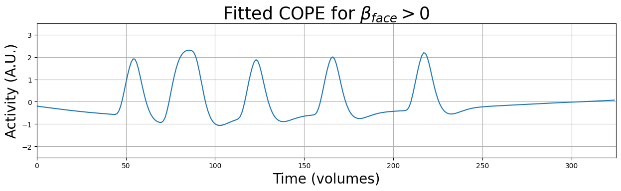
In the time series viewer, you should see a new line corresponding to “COPE1 fit: face”.
This is exactly the reason why we also defined the \(4\times\beta_{face} - \beta_{body} - \beta_{place} - \beta_{character} - \beta_{object} > 0\) contrast (contrast nr. 4 in our analysis)! This contrast allows us to identify regions in the brain that are (relatively more) specific for faces than for other types of images. In fact, in the context of our functional localizer task, you could argue that the \(\beta_{face} > 0\) contrast is largely useless.
Many voxels throughout the brain seem to specifically activate in response to images of faces (but beware: these brain images are not yet “properly” thresholded, so many of these voxels might actually be false positives, but that’s the topic of next week!). Two cluster of voxels, however, seem especially strongly activated: one centered at \([24, 19, 21]\) and another one centered at \([23, 30, 13]\). Note that these clusters are present in both hemispheres, but the cluster in the right hemisphere is clearly more strongly activated, which is consistent with the apparent right-hemisphere bias in face processing (see e.g., Kanwisher et al., 1997).
YOUR ANSWER HERE
This contrast shows you which voxels are more active during periods in which stimuli were absent than when stimuli were presented (regardless of condition). The pattern of voxels that are often found to be more active during “rest” than during (external) “stimulation” has been named the default mode network (DMN), which may reflect daydreaming, episodic or autobiographical information processing, or self reflection (amongst others; the exact “function” of the DMN is still unclear).
YOUR ANSWER HERE
This sigmasquareds map (and the underlying “raw” residual time series) can given you a good overview of the noise in your data and potential violations of GLM (e.g., unequal or correlated error variance). This is a great way to check for unexpected issues (e.g., artifacts) with your data, that will, if unmodelled, end up in your noise term.
This particular voxel lies most likely within the Circle of Willis: a “hub” of multiple arteries supplying blood to the brain. As BOLD MRI measures the (relative) amount of oxygenated blood in the brain, it is no surprise that arteries (and veins!) produce a strong heartbeat-related signal, which will, if left unmodelled, make up much of the unexplained variance. Indeed, in this sigmasquareds map, most of voxels with high values (i.e., those that are relatively yellow) are located within or near arteries or veins. For example, you can clearly “see” the sagittal sinus (see image below).
 From Wikimedia commons (link)
Apart from the veins/arteries, the cerebrospinal fluid (CSF) also seem to contain a lot of unmodelled noise. In fact, most of this unmodelled variance also likely represents the pulsative cerebral bloodflow, as shown (exaggerated) in the image below:

Now, move your crosshair across different voxels with high values (i.e., relatively yellow ones), for example voxel \([37, 48, 17]\) (located in the CSF). You can see that this voxel’s residual time series is highly (but not perfectly) correlated to the original voxel in the Circle of Willis, the common cause being the pulsative cerebral blood flow. (Note, though, that different voxels may show time series that look slightly shifted in time relative to the original Circle of Willis voxel, especially in more superior regions of the brain, which is caused by different slice onsets!)
Also note that the absolute signal amplitude of voxels within veins/arteries is much higher than voxels in gray matter!
Alright, time for something else: let’s delve into how you can “combine” run or session data in the next notebook (run_level_analyses.ipynb).