
Neurodesign (tutorial)#
In the previous tutorial, you have seen that jittered-ISI designs display quite some variance in efficiency (ranging from approx. 2.3 tot 3.1). This shows you that there are very many different designs possible, even with only two conditions, each associated with its own efficiency. Ideally, we want the best design (i.e., most efficient) out of all the possible designs. This is, however, for many (slightly more complex) designs not possible, because you would need to simulate billions of designs to exhaustively test them all! Moreover, we have also seen that high statistical efficiency (long blocked designs) may also have unwanted psychological effects (predictability, boredom).
So, how then should we look for (psychologically and statistically) efficient designs in the space of all possible designs? Fortunately, there exist methods to intelligently “search” for the optimal design among all possible designs without having to test them all and that allow you to define a balance between different aspects of your desired design.
Many different packages exist that implement this type of “design optimisation” (like optseq2, and the MATLAB toolbox by Kao). Here, we will give a short demonstration of the “neurodesign” toolbox; neurodesign is a Python package, but they offer also a web interface. Here, we will briefly walk you through the package. (Note that we use a slightly modified version of the original that works with Python3, which you can download here.)
import os
# Neurodesigninternally paralellizes some computations using multithreading,
# which is a massive burden on the CPU. So let's limit the number of threads
os.environ["OMP_NUM_THREADS"] = "1"
os.environ["OPENBLAS_NUM_THREADS"] = "1"
os.environ["MKL_NUM_THREADS"] = "1"

import numpy as np  # we'll also need Numpy
import neurodesign
The neurodesign package contains two important Python classes: the experiment class and the optimisation class. In the experiment class you define the most important parameters of your experiment.
First, we have to define the intended functional scan’s TR (let’s choose 1.6) and the expected degree of autocorrelation, rho, in the BOLD signal (we’ll discuss this in more detail next week; let’s set it to 0.6).
TR = 1.6
rho = 0.6
Now, more importantly, we have to define parameters related to the experimental conditions:
n_stimuli: the number of different stimulus conditions;n_trials: the number of different stimulus presentations per condition;duration: the duration of the experimental run (you can choose to set eithern_trialsorduration);stim_duration: the duration of each stimulus;P: the probability of occurring for each condition (e.g., [0.5, 0.5] for 50/50);t_pre: the time before the stimulus within each trial (e.g., fixation cross);t_post: the time after the stimulus within each trial (e.g., fixation cross; see image below);
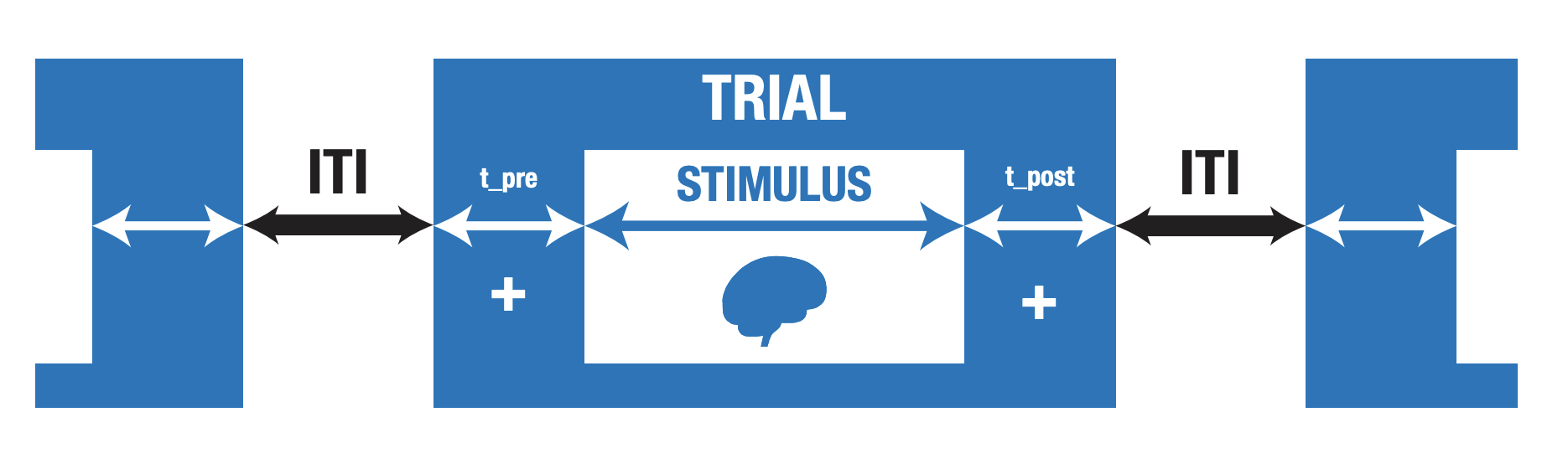 Image from the neurodesign preprint from Biorxiv
Now, let’s assume we our experiment is a simple “functional localizer”, in which we want to find brain regions that respond more strongly to faces than to houses. Now, we want those to conditions to occur equally often and have a stimulus duration of 2 seconds. We assume that we don’t want runs longer than 5 minutes (otherwise the participant might lose focus/fall asleep), so we’ll set the duration instead of the n_trials parameter. And we assume that there is a pre and post trial time of 0.1 seconds.
n_stimuli = 2
stim_duration = 1
duration = 5*60
P = [0.5, 0.5]
t_pre = 0.1
t_post = 0.1
Now, we have to define how neurodesign should create intertrial intervals (ITIs), the time between the offset of the previous trial and the onset of the next trial. In this package, you can specify a specific distribution and associated parameters from which these ITIs should be drawn (ITImodel). You can choose from "fixed", "uniform", and "exponential". Let’s pick "uniform" here, with a minimum ITI (ITImin) of 0.1 seconds and a maximum ITI (ITImax) of 8 seconds.
ITImodel = "uniform"
ITImin = 2
ITImax = 4
Lastly, we need to define the contrast(s) that we want to test (C). Let’s assume we want to test both “faces > houses” and “houses > faces”.
C = np.array([
    [1, -1],
    [-1, 1]
])
Now, with these parameters, let’s create an experiment object!
exp = neurodesign.experiment(
    TR=TR,
    rho=rho,
    n_stimuli=n_stimuli,
    stim_duration=stim_duration,
    P=P,
    duration=duration,
    t_pre=t_pre,
    t_post=t_post,
    ITImodel=ITImodel,
    ITImin=ITImin,
    ITImax=ITImax,
    C=C
)
Alright, now we need to create the optimisation object! This object defines how the experiment will be optimised. Neurodesign uses a “genetic algorithm” to efficiently look for the most efficient designs within the vast set of all possible designs, inspired by the way biological evolution works. We won’t go into the specifics of the algorithm.
The weights parameter of the optimisation class is very important: this allows you to balance different statistical and psychological aspects of your design. There are four aspects that can be optimized:
\(F_{e}\): the estimation efficiency (when you want to investigate the entire shape of the HRF);
\(F_{d}\): the detection efficiency (when you are only interested in amplitude changes/differences);
\(F_{f}\): how close the frequency of each condition is to the desired probability (given by
Pin theexperimentobject);\(F_{c}\): how well the conditions are “counterbalanced” in time. “Counterbalancing”, here, means that trying to make sure that each trial (\(n\)) has an equal probability to be followed by any condition (e.g., 50% condition A, 50% condition B for trial \(n+1\)), which can be extended to trials further in the future (\(n+2, n+3\), etc.). You can think of this parameter reflecting “predictability” (higher = less predictable).
Given that we’re only interested in detecting the difference between faces and houses, let’s set the weight for \(F_{d}\) to 1 and the rest to zero. Also, let’s tell neurodesign to save the best 10 designs (instead of only the very best) by setting the parameter outdes to 10. The other parameters (preruncycles, cycles, seed) are not important for now (but know that setting cycles, the number of iteration the algorithm runs for, to a higher number will increase the time it takes to run).
weights = [0, 1, 0, 0]  # order: Fe, Fd, Ff, Fc
outdes = 10

opt = neurodesign.optimisation(
    experiment=exp,  # we have to give our previously created `exp` object to this class as well
    weights=weights,
    preruncycles=10,
    cycles=1,
    seed=2,
    outdes=outdes
)
Now we can start the algorithm by calling the optimize method from the opt variable (this may take 5 minutes or so).
opt.optimise()
<neurodesign.classes.optimisation at 0x7fd1503b58e0>
Lastly, call the evaluate method to finalize the optimization run:
opt.evaluate()
<neurodesign.classes.optimisation at 0x7fd1503b58e0>
We can inspect the opt object, which now contains an attribute, bestdesign, that gives us the onsets (.onsets) and order (.order) of the best design found by the algorithm.
print("Onsets: %s" % (opt.bestdesign.onsets,), end='\n\n')
print("Order: %s" % (opt.bestdesign.order,))
Onsets: [  0.    3.9   7.4  11.6  16.3  19.9  23.8  27.2  31.3  34.7  38.3  41.6
  46.1  49.4  53.1  57.   61.7  65.2  69.6  74.5  78.7  83.9  87.5  92.4
  96.4  99.8 103.5 106.8 110.2 114.4 119.6 123.7 127.7 132.8 136.7 140.5
 145.5 149.1 152.4 155.7 160.3 164.6 169.3 173.9 178.7 182.  185.6 190.
 193.8 197.5 201.3 206.3 209.9 214.1 219.2 222.5 225.9 230.4 235.2 240.
 244.9 249.1 253.3 256.8 261.2 266.  269.5 273.1 277.9 282.3 286. ]

Order: [1, 1, 0, 0, 1, 1, 0, 0, 0, 1, 1, 1, 0, 0, 1, 1, 1, 1, 0, 0, 1, 1, 1, 1, 0, 0, 0, 1, 1, 0, 0, 1, 0, 0, 1, 1, 0, 0, 1, 1, 0, 0, 0, 1, 0, 0, 0, 1, 1, 0, 0, 0, 1, 1, 1, 0, 1, 0, 0, 1, 1, 1, 0, 1, 1, 0, 0, 0, 0, 1, 1]
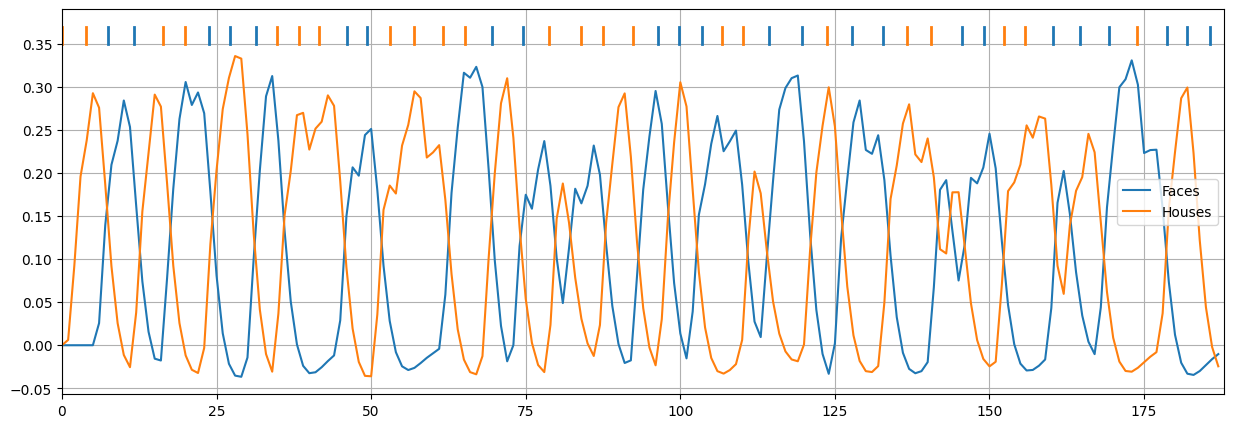
We even have access to the HRF-convolved design (Xconv; we’ll plot the onsets on top):
import matplotlib.pyplot as plt
%matplotlib inline

Xconv = opt.bestdesign.Xconv

plt.figure(figsize=(15, 5))
plt.plot(Xconv)
for ons, cond in zip(opt.bestdesign.onsets, opt.bestdesign.order):
    c = 'tab:blue' if cond == 0 else 'tab:orange'
    plt.plot([ons, ons], [0.35, 0.37], c=c, lw=2)

plt.legend(['Faces', 'Houses'])
plt.grid()
plt.xlim(0, Xconv.shape[0])
plt.show()
""" Try the ToDo here. """
' Try the ToDo here. '