
ROI analysis#
In the previous notebooks from this week, we’ve discussed how to implement “whole-brain” analyses: models that are applied to all voxels in the brain separately. As we’ve seen in the MCC notebook, this rather “exploratory” approach leads to issues of multiple comparisons, which are deceptively difficult to properly control for.
One alternative way to deal with the multiple comparisons problem is a more “confirmatory” approach: region-of-interest (ROI) analysis, which is the topic of this notebook.
What you’ll learn: after this lab, you’ll …
understand and implement ROI-based analyses (in Python)
Estimated time needed to complete: 1 hour
What is an ROI?#
An ROI is a prespecified brain region that is hypothesized to contain the hypothesized effects. These can be anatomically or functionally defined. Anatomical ROIs are regions of interest based on anatomical landmarks (such as folding pattern or histology), for example the caudate nucleus, inferior temporal gyrus, and anterior cingulate cortex.
As opposed to anatomical ROIs, functional ROIs are not based on anatomical properties, but on functional properties. These regions are usually determined on other, independent data and analyses. Sometimes, the data used for defining such a functional ROI comes from the same study, which acquired a so-called “functional localizer” in order to define a ROI for analysis of other data. This is also what we did in the NI-edu dataset: we acquired the floc runs in order to define functionally-defined “FFA” regions (based on the \(\beta_{face} > \mathrm{other}\) contrast) that can be used for ROI-analyses of the face perception runs (e.g., to answer questions like: does attractiveness of faces modulate FFA activity?).
In this section, we’ll show you how a typical ROI-analysis is done using an anatomical ROI. Then, the section after that will discuss how to derive functional ROIs within a single dataset.
An example ROI-analysis using an anatomical ROI#
For our anatomical ROI-analysis, we’ll stick to the flocBLOCKED data. Specifically, we will analyze the “face > other” contrast (i.e., \(4\cdot \beta_{face} - \beta_{place} - \beta_{body} - \beta_{character} - \beta_{object}\)) within the right amygdala (similar to this study). Our group-level hypothesis is that the amygdala activates significantly in response to faces (i.e., a one-sample, one-sided \(t\)-test):
\(H_{0}: \beta^{\dagger}_{face > other} = 0\)
\(H_{a}: \beta^{\dagger}_{face > other} > 0\)
The data that we load in below represents run-level \(c\hat{\beta}^{*}\) images corresponding to the “face > other” contrast from our 12 subjects. Data is in MNI152 (2 mm) space with voxel dimensions \([91, 109, 91]\).
import nibabel as nib
cope_4d_img = nib.load('contrast-faceGTother_level-run_stat-cope.nii.gz')
cope_4d = cope_4d_img.get_fdata()
print("Shape of data: %s" % (cope_4d.shape,))
Shape of data: (91, 109, 91, 12)
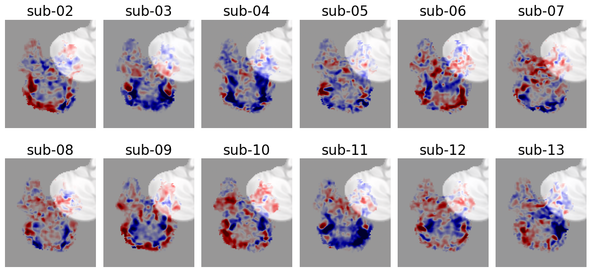
Let’s visualize this data. We’ll plot (using plt.imshow) a single (right-hemisphere) sagittal slice of each subjects’ COPE-image, with red indicating positive contrast-values (i.e., \(4\cdot \beta_{face} - \beta_{place} - \beta_{body} - \beta_{character} - \beta_{object} > 0\)) and blue indicating negative contrast-values (i.e., \(4\cdot \beta_{face} - \beta_{place} - \beta_{body} - \beta_{character} - \beta_{object} < 0\)).
import matplotlib.pyplot as plt
from nilearn.datasets import load_mni152_template
mni = load_mni152_template().get_fdata()

plt.figure(figsize=(12, 6))
subjects = ['sub-%s' % str(i).zfill(2) for i in range(2, 14)]

for i in range(cope_4d.shape[-1]):
    plt.subplot(2, 6, i+1)
    plt.title(subjects[i], fontsize=20)
    plt.imshow(mni[:, :, 26].T, origin='lower', cmap='gray')
    this_data = cope_4d[:, :, 26, i]
    plt.imshow(this_data.T, cmap='seismic', origin='lower',
               vmin=-500, vmax=500, alpha=0.6)
    plt.axis('off')
plt.tight_layout()
plt.show()
Now, conventional (exploratory) whole-brain analysis would fit a GLM on each voxel separately, but for our ROI-analysis, we’re going to do it differently: we’re only going to analyze the across-voxel average lower-level \(c\hat{\beta}^{*}\) values within the right amygdala.
We’ll load in the right amygdala mask first. This is a region from the probabilistic Harvard-Oxford subcortical atlas.
amygdala_probmask_img = nib.load('amygdala_lat-right_atlas-harvardoxford_thresh-0.nii.gz')
amygdala_probmask = amygdala_probmask_img.get_fdata()
print("Shape of probabilistic amygdala mask: %s" % (amygdala_probmask.shape,))
Shape of probabilistic amygdala mask: (91, 109, 91)
You have to do the following:
Create a boolean mask (array with True/False values) by tresholding the probabilitic mask at 20 (i.e., \(p(\mathrm{amygdala}) \geq 0.2\)). There should be 549 voxels surviving this threshold;
Average, per subject, the \(c\hat{\beta}^{*}\) values within this mask. You do not need a for-loop for this (hint: numpy broadcasting!);
Set up an appropriate group-level design matrix (\(\mathbf{X}^{\dagger}\)) that allows you to compute the average effect (\(\beta^{\dagger}\)) across the 12 ROI-average values (\(y^{\dagger}\)) and run a GLM;
With an appropriate group-level contrast, compute the \(t\)-value and \(p\)-value associated with our group-level hypothesis (outlined in the beginning of this section).
Store the ROI-average values (in total 12) as a numpy array in a variable named y_group, your group-level design matrix (a \(12 \times 1\) numpy array) in a variable named X_group, your group-level parameter (there should be only one) in a variabled named beta_group, and your \(t\)-value and \(p\)-value in variables named t_group and p_group respectively. You can use the stats.t.sf function to calculate the one-sided \(p\)-value from your \(t\)-value.
""" Implement the above ToDo here (step 1 and 2). """
import numpy as np

# YOUR CODE HERE
raise NotImplementedError()
''' Tests step 1 and 2. '''
from niedu.tests.nii.week_6 import test_roi_analysis_step1_step2
test_roi_analysis_step1_step2(amygdala_probmask, cope_4d, y_group)
""" Implement the above ToDo here (step 3). """

# YOUR CODE HERE
raise NotImplementedError()
''' Tests step 3. '''
from niedu.tests.nii.week_6 import test_roi_analysis_step3
test_roi_analysis_step3(y_group, X_group, beta_group)
""" Implement the above ToDo here (step 4). """
from scipy import stats

# YOUR CODE HERE
raise NotImplementedError()
''' Tests step 4 (t_group, p_group). '''
from niedu.tests.nii.week_6 import test_roi_analysis_step4
test_roi_analysis_step4(y_group, X_group, beta_group, t_group, p_group)
Functional ROIs & neurosynth#
In addition to anatomical ROIs, you can also restrict your analyses to functionally defined ROIs. “Functionally defined”, here, means that the region has been derived from or determined by its assumed function. This can be done using a (separate) dataset specifically designed to localize a particular functional region (the “functional localizer” approach). Another option is to define your ROI based on a meta-analysis on a particular topic. For example, you could base your ROI on (a set of) region(s) on a meta-analysis of the neural correlates of face processing.
One particular uesful tool for this is neurosynth (see also the associated article). Neurosynth is a tool that, amongst other things, can perform “automatic” meta-analyses of fMRI data. As stated on its website, “it takes thousands of published articles reporting the results of fMRI studies, chews on them for a bit, and then spits out images” that you can use, for example, a functional ROIs.
Now, click on the term “emotional faces”.
After selecting a particular term, Neurosynth will open a new page with an interactive image viewer. By default, it shows you the result (i.e., \(z\)-values) of an “association test” of your selected term across voxels, which tests whether voxels are preferentially related to your selected term (click on “FAQs” for more information).
Conduct a meta-analysis using the term “reward”, set the threshold to \(z > 12\) (note that this exact value is somewhat arbitrary; make sure to decide on this cutoff before looking at your own data as to avoid circularity in your analysis!). Download this thresholded map by clicking on the download symbol (next to the trash bin icon) next to “reward: association test”. This will download a nifti file to your own computer.
If you’re working on a Jupyterhub instance, upload this image as follows:
Under the “Files” tab in Jupyterhub, navigate to your week_6 folder (with your mouse);
Click on the “Upload” button, select the downloaded file (reward_association-test_z_FDR_0.01.nii.gz), and click on the blue “Upload” button to confirm.
''' Tests the ToDo above. '''
import os.path as op
here = op.abspath('')
par_dir = op.basename(op.dirname(here))

if par_dir != 'solutions':  # must be student account
    try:
        assert(op.isfile('reward_association-test_z_FDR_0.01.nii.gz'))
    except AssertionError:
        msg = "Could not find 'reward_association-test_z_FDR_0.01.nii.gz' file!"
        raise ValueError(msg)
    else:
        print("Well done!")
Although slightly off-topic, another great Neurosynth functionality is its “decoder”. As opposed to its meta-analysis functionality which generates the most likely (and specific) brain map given a particular term, the decoder produces the most likely terms given a particular (untresholded) brain map! This is great way to help you interpret your (whole-brain) results (but this does not replace a proper and rigorous experimental design).
In this week’s directory (week_6), we included the unthresholded \(z\)-value map from the group-level (mixed-effects) analysis of the \(4\cdot \beta_{face} - \beta_{place} - \beta_{body} - \beta_{character} - \beta_{object}\) contrast: contrast-faceGTother_level-group_stat-zstat.nii.gz. You need to download this file to your computer, which you can do by navigating to your week_6 directory in Jupyterhub, selecting the file, and clicking on “Download”. Now, let’s decode this image.
After registration on the Neurovault website, you should be redirected to a short “questionnaire” where you have to fill in some metadata associated with the image. Give it a name (e.g., “FFA localizer”), add it to a particular “collection” (“{your username} temporary collection” is fine), set the map type to “Z map”, set the modality & acquisition type to “fMRI-BOLD”, and “Cognitive Atlas Paradigm” to “face recognition task” (this is unimportant for now). Finally, under “File with the unthresholded volume map”, select the just downloaded file and click “Submit” at the very bottom.
You should be redirected to “Neurosynth”, which should now visualize our group-level “face > other” \(z\)-statistic file. Now, at the bottom of the page, you find a table with “Term similarity”, showing the terms whose unthresholded brain maps correlate the most with our just uploaded brain map. Scrolling through these terms, you’ll notice a lot of terms associated with the “default mode network” (DMN)! We are not sure why our “face map” correlates so highly with the brain map typically associated with the DMN … One reason might be that faces deactivate the DMN less than the other conditions (bodies, places, etc.), which shows up as a positive effect in the “face > other” contrast.
Alright, let’s get back to the topic of functional ROIs again. Given that you defined a functional ROI, the process of analyzing your data proceeds in the same fashion as with anatomical ROIs:
You average your lower-level data (\(c\hat{\beta}^{*}\)) within your ROI;
You construct a group-level design matrix and run a GLM;
Proceed as usual (construct group-level contrats, calculate \(t\)/\(z\)-values, etc.)
The end!#
You finished the last (mandatory) notebook! If you want, there are two optional notebooks next week, in which you can try out the functionality of the awesome Nilearn package.
print("Well done!")
Well done!