Machine learning (“decoding”) analyses

Machine learning (“decoding”) analyses#

This week’s tutorial is about how to implement “decoding” analyses in Python!

The term “decoding” is often used to denote analyses that aim to predict a single experimental feature (which can be either within-subject or between-subject) based on patterns of neuroimaging data. Some more advanced techniques make it possible to predict more than one experimental feature at once (with Bayesian “reconstruction” techniques and “inverted encoding models”), but these are beyond the scope of this course. Here, we’ll focus on machine learning/statistical models and techniques that allow you to predict a single experimental feature.

We’ll make heavy use of the awesome scikit-learn library — the go-to library for machine learning in Python.

What you’ll learn: at the end of this tutorial, you will be able to:

use and implement feature-selection/extraction methods;
fit machine learning models and predict (new) samples;
implement cross-validation routines;
statistically evaluate model performance estimates;

Estimated time needed to complete: 8-12 hours
Credits: if you use scikit-learn in your research, please cite the corresponding paper

Data representation#

Decoding analyses always need two sets of data: the brain patterns, which we’ll refer to as $\mathbf{R}$ (for Response), and a single experimental feature that we want to predict, which we’ll refer to as $\mathbf{S}$ (which traditionally refers to Stimulus). Note that $\mathbf{s}$ could be a within-subject experimental factor (such as stimulus or response-related factors) or a between-subject variable (such as age or depressed vs. healthy control). Moreover, the to-be-predicted variable* can be either continuous (e.g., reaction time) or categorical (e.g., object category), which are associated with different types of models, regression and classification models respectively (more about this later). Note that “direction” of analysis is the exact opposite of what is done in enconding analyses. In encoding analyses, we try to predict the brain data (dependent variable) using experimental features (independent variables), while in decoding analyses we try to predict an experimental feature (dependent variable) using a a set of brain patterns (independent variables)! But essentially, encoding and decoding models are mathematically the same (they just use different inputs).

In the first part of this lab, we’ll work with simulated data. For now, we’ll assume that our data is from a simple face perception experiment in which participants viewed images with either male (condition: “M”) or female faces (condition: “F”) across four different fMRI runs. So, our experimental feature of interest is a categorical variable with two levels (“M” and “F”), making this a classification analysis (which is more common than regression in the context of cognitive neuroscience). Each run, participants saw fourty images (twenty for each condition) presented in a random order.

We’ll simulate the patterns ($\mathbf{R}$) and experimental feature ($\mathbf{S}$, “M” vs. “F”) below. For now, we’ll generate random data (with some autocorrelation), for reasons that will become clear later. We’ll assume that we are restricting our analysis to a single region-of-interest containing a 1000 voxels.

* Often, the to-be-predicted variable is called the “target” or “dependent variable”. Here, we’ll use the term “target”.

import numpy as np
from scipy.linalg import toeplitz
from niedu.utils.nipa import generate_labels

N_per_run = 40
M = 4  # nr of runs
K = 1000  # nr of voxels

# Generate random data drawn for a multivariate normal
# distribution with AR1 noise (with phi = 0.85) to
# simulate autocorrelated noise in the estimated patterns,
# which is plausible for designs with relatively short ISIs
mu = np.zeros(N_per_run)
V = 0.85 ** toeplitz(np.arange(N_per_run))

# R_runs is a list of M arrays of shape N_per_run x K
R_runs = [np.random.multivariate_normal(mu, V, size=K).T for _ in range(M)]

# S_runs is a list of M arrays of shape N_per_run
# The custom generate_label function creates slightly correlated
# labels
S_runs = [generate_labels(['M', 'F'], N_per_run / 2, [0.7, 0.3]) for _ in range(M)]

print("Example of patterns for run 1:\n", R_runs[0])
print("\nExample of target for run 1:\n", S_runs[0])

Example of patterns for run 1:
 [[ 0.70248736 -0.94395733 -0.51906461 ...  1.02065335 -0.5481945
  -0.70312707]
 [ 0.63195884 -0.87853903 -0.30651633 ...  1.66633316 -0.44055865
  -0.15091501]
 [ 2.06738308 -0.981851   -0.90944086 ...  1.47832213  0.75926163
  -0.4902048 ]
 ...
 [-0.02752864 -0.34174816 -2.05763914 ...  0.30884591 -0.26293549
  -0.86723688]
 [ 0.62627232 -0.10885171 -3.02955439 ... -0.35126472 -0.94343858
  -1.56204958]
 [ 0.46080567 -0.029      -1.34808462 ... -0.55228256 -0.13795203
  -0.63026681]]

Example of target for run 1:
 ['M', 'F', 'F', 'M', 'M', 'F', 'F', 'M', 'M', 'M', 'F', 'F', 'F', 'M', 'M', 'M', 'M', 'M', 'F', 'M', 'M', 'F', 'F', 'F', 'F', 'F', 'F', 'M', 'M', 'M', 'M', 'M', 'M', 'M', 'F', 'F', 'F', 'F', 'F', 'F']

Alright, technically, we have everything we need for a decoding analysis. However, machine learning (ML) and statistical models often require all data to be represented numerically, so we need to convert our target (containing the values “M” and “F”) into a numeric format.

ToDo (optional; 0 points): If you want to practice your Python skills, try converting the string labels of run 1 (the S_run1 variable below) to numeric labels. Specifically, use the integer 0 for trials of condition "F" and the integer 1 for trials of condition "M". Store the result in a new variable called S_run1_num; make sure it's a numpy array. (To convert a list to a numpy array, you can do: np.array(your_list) ).

S_run1 = S_runs[0]

# YOUR CODE HERE
raise NotImplementedError()

''' Tests the above ToDo. '''
from niedu.tests.nipa.week_2 import test_lab2num
test_lab2num(S_run1, S_run1_num)

While converting labels to numeric values can be done quite easily using standard Python, it gives us with a nice excuse to introduce some scikit-learn functionality. Specifically, the LabelEncoder class, which allows you to encode your target labels into a numeric format. Let’s start with importing it (from the preprocessing module):

from sklearn.preprocessing import LabelEncoder

The way LabelEncoder is used is similar to some of the Nilearn and Nistats functionality you’ve seen. In short, you first need to initialize the object (with, optionally, some parameters), after which you can give it data to fit and transform. This pattern is something we’ll encounter a lot in this lab when working with scikit-learn.

Let’s initialize a LabelEncoder object below:

# LabelEncoder objects are not initialized with any parameters
lab_enc = LabelEncoder()

Now, let’s “fit” it on the labels of our first run:

lab_enc.fit(S_runs[0])

LabelEncoder()

In a Jupyter environment, please rerun this cell to show the HTML representation or trust the notebook.
On GitHub, the HTML representation is unable to render, please try loading this page with nbviewer.org.

Notice that the fit function doesn’t return anything useful (well, technically, it returns itself). Instead, when calling fit, it stores some parameters in the object itself as attributes which are used when calling the transform. For the LabelEncoder specifically, it stores the unique conditions (often called classes in machine learning) in an attribute called classes_:

print(lab_enc.classes_)

['F' 'M']

In general, most “things” that are inferred or computed in the fit method of scikit-learn objects (and are needed later when calling transform) are stored in attributes with a trailing underscore (like classes_). We know, this all sounds incredibly trivial, but explaning these things in detail will give you a better understanding of how scikit-learn works (which is going to help a lot when dealing with more complicated functionality).

Finally, after fitting the LabelEncoder object, we can call the transform method to actually transform the labels:

S_run1_num = lab_enc.transform(S_runs[0])
print(S_run1_num)

[1 0 0 1 1 0 0 1 1 1 0 0 0 1 1 1 1 1 0 1 1 0 0 0 0 0 0 1 1 1 1 1 1 1 0 0 0
 0 0 0]

Note that, unlike the fit method, the transform method actually returns something, i.e., the transformed labels. Also note that the numeric labels are assigned alphabetically (i.e., “F” gets assigned 0, “M” gets assigned 1).

Like you’ve seen in the Nilearn notebook, we can often call fit and transform at once using the fit_transform method:

S_run1_num = lab_enc.fit_transform(S_runs[0])
print(S_run1_num)

[1 0 0 1 1 0 0 1 1 1 0 0 0 1 1 1 1 1 0 1 1 0 0 0 0 0 0 1 1 1 1 1 1 1 0 0 0
 0 0 0]

Also, after the LabelEncoder has been fit, it can be reused on other data, i.e., you can call the transform method on new arrays. This is how many classes in scikit-learn are actually used (i.e., fit on a particular subset of data and then apply to another subset), as it allows for efficient cross-validation &mdash a topic that will discuss in detail later.

ToDo (1 point): We just converted the labels from the first run only. For this ToDo, convert the labels from all runs (i.e., the S_runs variable) using the LabelEncoder. Store the results in a new variable named S_runs_num, which should be a list (of length four, i.e., four runs) of arrays with ones and zeros (instead of "M" and "F").

''' Implement your ToDo here . '''
# YOUR CODE HERE
raise NotImplementedError()

''' Tests the above ToDo. '''
from niedu.tests.nipa.week_2 import test_lab2num_all_runs   
test_lab2num_all_runs(S_runs, lab_enc, S_runs_num)

Alright, now we have everything we need to start building our decoding pipeline!

Standardization#

In addition to the “preprocessing” steps for pattern analyses discussed in last week’s lab, when doing decoding, you additionally need to standardize your brain features (i.e., the columns in your pattern matrix) on which you fit your model. With “standardization”, we mean making sure each feature ($\mathbf{R}_{j}$ for column $j$) in your pattern matrix has 0 zero mean and unit (1) standard deviation, which can be achieved as follows for each feature $j$:

(92)#\[\begin{align} \mathbf{R}_{j, norm} = \frac{\mathbf{R}_{j} - \bar{\mathbf{R}}_{j}}{\hat{\sigma}(\mathbf{R}_{j})} \end{align}\]

where $\bar{\mathbf{R}_{j}}$ represents the mean of $\mathbf{R}_{j}$ and $\hat{\sigma}(\mathbf{R}_{j})$ represents the standard deviation of $\mathbf{R}_{j}$. In other words, for each value in $\mathbf{R}$, you subtract the mean from the column it belongs to and subsequently you divide the result by the standard deviation of the column it belongs to. This process is also known as z-scoring.

This standardization process is done for each brain feature (column) separately. Standardization is important for most ML/statistical models because it makes sure that each brain feature has the same scale, which often helps in efficiently estimating model parameters.

Importantly, when you have patterns from multiple runs (as is often the case in fMRI decoding), these patterns should also be independently standardized, even if you want to pool these patterns later on (see Lee & Kable, 2018). This is because some runs may yield patterns with a relatively higher mean or standard deviation across samples (for example, because participants start moving more towards the end of the experiment, leading to more noisy pattern estimates).

ToDo (1 point): In this ToDo, you have to standardize the data from run 1 (the R_run1 variable below) using Numpy (afterwards, we'll show you how to do this using scikit-learn). Store the results (which should have columns with mean zero and unit standard deviation) in a new variable called R_run1_norm. Importantly, this can be done efficiently (without a for-loop) using broadcasting!

''' Implement your ToDo here. '''
R_run1 = R_runs[0]

# YOUR CODE HERE
raise NotImplementedError()

''' Tests the ToDo above. '''
# ToThink: do you understand how we're testing your answer here?
np.testing.assert_array_almost_equal(R_run1_norm.mean(axis=0), np.zeros(R_run1.shape[1]))
np.testing.assert_array_almost_equal(R_run1_norm.std(axis=0), np.ones(R_run1.shape[1]))
print("Well done!")

We can do this similarly using the StandardScaler class from scikit-learn, which has the same fit/transform interface:

from sklearn.preprocessing import StandardScaler
scaler = StandardScaler()
R_run1_norm = scaler.fit_transform(R_run1)

In the fitting process, the StandardScaler computed the feature-wise mean and standard deviation, which it stores in the mean_ and _scale attributes:

print(scaler.mean_.shape)
print(scaler.scale_.shape)

(1000,)
(1000,)

For the initial run-wise standardization, we usually don’t want to cross-validate our standardization process (i.e., to for example fit the StandardScaler on run 1 and subsequently transform the other runs) for reasons discussed before. As such, we need to call fit and transform on each run separately:

# Below, we use a "list comprehension" to loop across our runs
# to standardize each run separately!
R_runs_norm = [scaler.fit_transform(this_R) for this_R in R_runs]

We’re almost ready to start fitting models. Before we do so, we are going to concatenate our data ($\mathbf{R}$ and $S$) across runs because we want to give our model as much data as possible!

# Load S_runs_num if you didn't manage to do the last ToDo
S_runs_num = np.load('S_runs_num.npy')

R_all = np.vstack(R_runs_norm)  # stack vertically
S_all = np.concatenate(S_runs_num)

print("Shape R_all:", R_all.shape)
print("Shape S_all:", S_all.shape)

Shape R_all: (160, 1000)
Shape S_all: (160,)

Fitting models#

When fitting decoding models, we assume that we can approximate our target variable ($\mathbf{S}$) as a function of the input data ($\mathbf{R}$):

(93)#\[\begin{align} \hat{\mathbf{S}} \approx f(\mathbf{R}) \end{align}\]

Usually, the models used in pattern analyses assume linear functions (especially with relatively little data), i.e., functions that approximate the target using a linear combination of input variables ($\mathbf{R}_{j}$) weighted by parameters ($\beta$). Note that the univariate GLM often used in encoding models is such a linear model. The process of model fitting is estimating parameters that minize the discrepancy (error) between the predicted values ($\hat{\mathbf{S}}$) and the actual values ($\mathbf{S}$) of the target variable, both for regression ($\mathbf{S}$ is continuous) and classification ($\mathbf{S}$ is categorical) models. Different models differ in how they exactly estimate their parameters, but the general process is the same (minimizing error between predictions and target). In this course, we won’t go much into the differences across models (partly because in practice, we found that performance doesn’t differ that much between models).

Alright, let’s get to it. Below, we import the LogisticRegression class, a particular linear classification model (unlike the name suggests).

from sklearn.linear_model import LogisticRegression

We are many “options” (often called “hyperparameters”) we can set upon initialization of a LogisticRegression object, but for now, we will only set the “solver” (for no other reason that this will get rid of a warning during the fitting process):

# clf = CLassiFier
clf = LogisticRegression(solver='lbfgs')

Now, the fitting process using this model (or actually, any model in scikit-learn) is as simple as, guess what, calling the fit method! Unlike the LabelEncoder and StandardScaler that we discussed before, models in scikit-learn (including LogisticRegression) require two arguments when calling their fit method: X and y, which represent the input data (in our case: $\mathbf{R}$) and the target variable (in our case: $\mathbf{S}$):

# The text in the output cell is there because the
# fit model returns "itself" (you can just ignore this)
clf.fit(R_all, S_all)

LogisticRegression()

In a Jupyter environment, please rerun this cell to show the HTML representation or trust the notebook.
On GitHub, the HTML representation is unable to render, please try loading this page with nbviewer.org.

After fitting, the model stores the estimated parameters ($\beta$) as an araay in the coef_ (“coefficients”, another term for parameters) attribute:

print("Shape of coef_:", clf.coef_.shape)

Shape of coef_: (1, 1000)

As you can see, the model estimated one parameter for each brain feature (column in $\mathbf{R}$). Now, unlike the previously discussed LabelEncoder and StandardScaler, scikit-learn models do not have a transform method; instead, they have a predict method, which takes a single input (a 2D array with observations) and generates discrete* predictions for this input. For now, we’ll call predict on the same data we’ve fit the model on:

* Some models, including the LogisticRegression model, have an additional method called predict_proba which returns probabilistic instead of discrete predictions.

preds = clf.predict(R_all)
print("Predictions for samples in R_all:\n", preds)

Predictions for samples in R_all:
 [0 0 0 0 1 1 0 0 1 1 1 1 1 1 1 1 1 1 0 1 1 1 1 0 1 0 1 1 1 0 0 0 0 0 0 0 0
 0 0 0 1 1 0 0 1 1 0 0 1 1 1 1 1 0 1 0 0 0 0 0 0 0 0 1 0 0 0 0 0 0 0 1 1 1
 1 1 1 1 1 1 0 1 0 0 0 0 1 1 1 0 0 0 1 0 0 0 1 1 1 1 1 1 1 1 1 1 0 0 0 1 1
 1 0 0 1 0 1 0 0 0 1 1 0 0 1 1 1 0 0 0 1 1 1 1 0 1 1 1 1 1 1 1 1 1 1 1 0 0
 0 0 0 0 0 0 0 0 0 0 0 0]

Model evaluation#

Alright, we have some preditions for our data! But how do we evaluate these predictions? This actually depends on whether you have a classification model (with categorical predictions) or a regression model (with continuous predictions). Because classification analyses are most popular in cognitive neuroscience (and our example data is categorical) and you are already familiar with some regression metrics such as $R^2$ (discussed in the previous course), we’ll focus on model evaluation metrics for classification here.

Metrics for discrete predictions#

There are many different metrics to evaluate the predictions of classification models. The most well known (but not necessarily always appropriate) metric for discrete predictions is accuracy, which is defined as follows:

(94)#\[\begin{align} \mathrm{accuracy} = \frac{\mathrm{number\ of\ correct\ predictions}}{\mathrm{total\ number\ of\ predictions}} \end{align}\]

For accuracy, the best possible score is 1 (predict all samples correctly) and “chance level” performance (i.e., the expected score when randomly guessing) is, in general, $\frac{1}{\mathrm{Number\ of\ classes}}$, so for our example with two classes (“M” and “F”), it is 0.5.

ToDo (1 point): Using the predictions (the preds variable) and the true labels (the S_all variable), compute the associated accuracy and store this in a variable acc. Note: there is no need for a for-loop! You can use the fact that boolean values, True and False, evaluate to 1 and 0, respectively, in Python...

''' Implement your ToDo here. '''
# YOUR CODE HERE
raise NotImplementedError()

''' Tests the above ToDo. '''
from niedu.tests.nipa.week_2 import test_acc
test_acc(preds, S_all, acc)

Metrics for probabilistic predictions#

Some classifiers allow for probabilistic (instead of discrete) predictions. For those classifiers, an additional method called predict_proba exists, which outputs a probability for each class. So, in a two-class classification setting, the predict_proba method will not give a single discrete prediction (i.e., either 0 or 1) but a probability distribution over classes (e.g., 0.92 for class 0 and 0.08 for class 1).

The LogisticRegression model from scikit-learn actually allows for probabilistic prediction. In general, if we’ll give it all $N$ trials for a target variable with $M$ classes, it will output a $N \times M$ array with probabilities:

probas = clf.predict_proba(R_all)
# let's print the first five trials
print(np.round(probas[:5, :], 3))

[[0.994 0.006]
 [0.998 0.002]
 [0.996 0.004]
 [0.989 0.011]
 [0.013 0.987]]

One often-used performance metric for probabilistic predictions is the “Area Under the ROC curve” (often abbreviated as AUROC or just AUC). Fortunately, the scikit-learn library contains implementations of many performance metrics, including AUROC (called roc_auc_score in scikit-learn), which can be imported from the metrics module:

from sklearn.metrics import roc_auc_score

AUROC is an excellent metric to use for probabilistic predictions, but there’s one caveat: when evaluating probabilistic predictions (formatted as a $N \times M$ matrxi), it needs the true target values (dependent variable) in a one-hot-encoded format. One-hot-encoding (OHE) is a technique that transforms a $N \times 1$ vector with $M$ classes into a $N \times M$ binary matrix:

(95)#\[\begin{align} S = \begin{bmatrix} 1 \\ 2 \\ 1 \\ 3 \\ 2 \\ 4 \end{bmatrix} \underset{\Longrightarrow}{\mathrm{OHE}} \begin{bmatrix} 1 & 0 & 0 & 0 \\ 0 & 1 & 0 & 0 \\ 1 & 0 & 0 & 0 \\ 0 & 0 & 1 & 0 \\ 0 & 1 & 0 & 0 \\ 0 & 0 & 0 & 1 \end{bmatrix} \end{align}\]

You might know this technique under the name “dummy (en)coding”.

ToDo (optional): Complete the one_hot_encode function below that takes in a 1D vector representing a target variable with any number of classes and observations and outputs a one-hot-encoded version of that target variable.

''' Implement the optional ToDo here. '''

def one_hot_encode(y):
    ''' One-hot-encodes a 1D target vector. 
    
    Parameters
    ----------
    y : numpy array
        1D target vector with N observations and M classes
    
    Returns
    -------
    An NxM numpy array
    '''
    # YOUR CODE HERE
    raise NotImplementedError()

''' Tests the above ToDo. '''
# Test 1
y = np.array([0, 1])
out = one_hot_encode(y)
ans = np.eye(2)
np.testing.assert_array_equal(ans, out)

# Test 2
y = np.array([1, 2, 3, 2, 2, 1])
out = one_hot_encode(y)
ans = np.array([[1, 0, 0], [0, 1, 0], [0, 0, 1], [0, 1, 0], [0, 1, 0], [1, 0, 0]])
np.testing.assert_array_equal(ans, out)

# Test 3
y = np.array([3, 2, 1])
out = one_hot_encode(y)
ans = np.rot90(np.eye(3))
np.testing.assert_array_equal(ans, out)

print("Well done!")

While the above ToDo was a nice way to practice your Python skills, we nonethless recommend using the OneHotEncoder class from scikit-learn to one-hot-encode your target vector. It uses the fit-transform syntax you are familiar with by now. Importantly, as the OneHotEncoder is, in practice, often used to one-hot-encoded predictors (independent variables), it expects a 2D array (not a 1D vector). So, when one-hot-encoding a 1D target variable, you can add a singleton axis (with np.newaxis) to make it work:

from sklearn.preprocessing import OneHotEncoder
ohe = OneHotEncoder(sparse_output=False)  # we don't want a "sparse" output
S_all_ohe = ohe.fit_transform(S_all[:, np.newaxis])
print(S_all_ohe.shape)

(160, 2)

Finally, we can use the roc_auc_score function to compute our model performance. Like any metric implementation in scikit-learn, it is called as follows:

score = metric(true_labels, predicted_labels)

where true_labels and predicted_labels are either 1D vectors of length $N$ (in case of discrete predictions) or 2D $N \times M$ arrays (in case of probabilistic predictions). Note that by default these metrics output a single score (often the average of the class-specific scores); some (but not all) metrics (including the roc_auc_score) allow the function to return a class-specific score by setting the optional argument average to None:

# Omit average=None to get a single (average) score
scores = roc_auc_score(S_all_ohe, probas, average=None)
print(scores)

[1. 1.]

ToDo (optional, quite difficult!): Another class of classification metrics are "pseudo $R^2$" scores. These metrics are similar to $R^2$ in regression models in the sense that they are bounded between 0 (chance performance) and 1 (perfect performance). They often assume probabilistic predictions.

One of these pseudo $R^2$ metrics is “Tjur’s pseudo $R^2$” which is defined as the difference between the average (across observations) probability of a particular class and the average probability of the other class(es) for a given label. So, suppose we’re dealing with a two-class classification problem (with class 0 and class 1), and the average probability for class 1 of trials belonging to class 1 is 0.9, while the average probability for class 1 of trials belonging to class 0 is 0.3, then the Tjur’s pseudo $R^2$ score for class 1 is $0.9-0.3=0.6$. Formally, the Tjur’s pseudo $R^2$ score for class $m$ is defined as:

(96)#\[\begin{align} R^2_{m} = \frac{1}{N}\sum_{i=1}^{N}p(\hat{s}^{m}_{i}) - \frac{1}{N}\sum_{i=1}^{N}p(\hat{s}^{\neg m}_{i}) \end{align}\]

for any set of trials belonging to class 1 ($p^{m}_{i}$) and complementary set of trials not beloning to class 1 ($p^{\neg m}_{i}$).

Complete the function tjur_r2 below that takes two arguments — target (a 1D array with target labels) and probas (a 2D array with probabilities) — and should output an array of length $M$ with Tjur’s pseudo $R^2$ scores for the $M$ classes in the target array.

''' Implement your ToDo here. '''

def tjur_r2(target, probas):
    ''' Computes Tjur's R2 score for all classes in `target`.
    
    Parameters
    ----------
    target : numpy array
        A 1D array with numerical targets
    probas : numpy array
        A 2D array with target probabilities
    
    Outputs
    -------
    A numpy array of length M with R2 scores for all M classes
    '''
    
    # YOUR CODE HERE
    raise NotImplementedError()

''' Tests the ToDo above. '''
y = np.array([0, 0, 1, 1])
probas = np.array([[0.9, 0.1], [0.95, 0.05], [0.3, 0.7], [0.4, 0.6]])
ans = tjur_r2(y, probas)
np.testing.assert_array_almost_equal(ans, np.array([0.575, 0.575]))

y = np.array([1, 1, 3, 3, 2, 2])
probas = np.array([[0.8, 0.1, 0.1], [0.7, 0.2, 0.1], [0.4, 0.0, 0.6], [0.3, 0.1, 0.6], [0.1, 0.5, 0.4], [0.2, 0.6, 0.2]])
ans = tjur_r2(y, probas)
np.testing.assert_array_almost_equal(ans, np.array([0.5, 0.45, 0.4]))
print("Well done!")

Tip: This article by Dinga and colleagues (2019) argues against "accuracy" as a performance metric for classification models and reviews several (often probabilistic) alternatives; a highly recommended read!

Cross-validation#

If you did the previous ToDos correctly, you should have found that the accuracy was 1 (the maximum possible score)! Amazing! But wait, how is this possible? We generated random data, right?

So, what is the issue here? Well, we fitted the model on the same data that we want to generate predictions for! While this is common practice in many statistical models in psychology and neuroscience (including standard univariate “activation-based” fMRI models), this is not advisable for decoding models. The reason for this is that our decoding models often have many more predictors (i.e., brain features) than observations (i.e., trials). The consequence is that the model has a hard time figuring out what is “signal” and what is “noise”, which will often cause your model to capitalize on spurious correlations between your data ($\mathbf{R}$) and the target ($\mathbf{S}$). The result is that your model will be overfitted and your model performance estimate will be overly optimistic estimate of generalization performance.

To obtain an unbiased (that is, not overly optimistic) estimate of generalization performance, machine-learning based analyses often perform cross-validation. Cross-validation is, in it’s broadest definition, the process of estimating analysis parameters on a different subset of your data than the data you want to generate predictions for (and thus base generalization performance on). With “analysis parameters”, we do not only mean the parameters of your statistical model ($\hat{\beta}$), but this may also involve parameters estimated during preprocessing and feature transformations (which we’ll talk about later). Importantly, cross-validation (if done properly) allows you to derive an unbiased estimate of generalization performance, i.e., how well your analysis would generalize to a new dataset. Importantly, cross-validation does not solve overfitting; it only detects overfitting. To prevent overfitting, you can employ regularization or feature selection/extraction techniques, of which the latter is briefly discussed in this tutorial.

Train vs. test set partitioning#

Usually, the subset of data you use to fit your analysis parameters on is called the train set and the subset you evaluate your model predictions on is often called the test set. Assuming that each observation (i.e., row in $\mathbf{R}$) is independent from all other observations, any spurious correlation that is capitalized upon in the train set will not generalize to the test set!

There are different cross-validation schemes (i.e., how you partition your data in a train and set set). For the example in the next cell, we’ll use a simple hold-out scheme, in which we’ll reserve 50% of the data for the test set (note that this could have been a different percentage). (We’ll discuss more intricate cross-validation schemes such as K-fold in the next section).

R_train = R_all[0::2, :]  # all even samples
S_train = S_all[0::2]

R_test = R_all[1::2, :]  # all odd samples
S_test = S_all[1::2]

After splitting the data into a train and test set, we have introduced a “problem” however: the features within the train and test set may not have 0 mean and unit (1) variance anymore! Given that the features were properly standardized across all samples in our simulated fMRI dataset, this is unlikely to be a problem for our classifier. It is still good practice to make sure your train set is properly standardized. So, before fitting our classifier, let’s standardize the train set:

R_train_norm = scaler.fit_transform(R_train)

Now, we can fit our model on the standardized train set …

clf.fit(R_train_norm, S_train)

LogisticRegression()

In a Jupyter environment, please rerun this cell to show the HTML representation or trust the notebook.
On GitHub, the HTML representation is unable to render, please try loading this page with nbviewer.org.

Before predicting the test set, however, we need to decide whether we want to independently standardize the test set or whether to cross-validate our previously estimated standardized parameters (the feature-wise mean and standard deviation). Although opinions differ on this topic (see e.g. this excellent article), if we want a truly unbiased estimate of generalization, we should also cross-validate our standardization procedure in addition to cross-validation of our model. So, to cross-validate our standardization procedure, we do the following for each feature $j$ of our test set:

(97)#\[\begin{align} \mathbf{R}_{j, norm}^{\mathrm{test}} = \frac{\mathbf{R}_{j}^{\mathrm{test}} - \bar{\mathbf{R}}_{j}^{\mathrm{train}}}{\hat{\sigma}(\mathbf{R}_{j}^{\mathrm{train}})} \end{align}\]

# Note that we're *not* calling fit on the test set, i.e.,
# we're cross-validating our standardization procedure!
R_test_norm = scaler.transform(R_test)

So, now we can cross-validate our model and derive predictions for our test set:

preds = clf.predict(R_test_norm)
print("Predictions for our test set samples:\n", preds)

Predictions for our test set samples:
 [0 0 1 1 1 1 1 1 1 1 1 1 1 1 1 0 0 0 0 0 1 1 0 1 1 1 1 1 0 0 0 0 0 0 0 0 1
 1 1 1 0 0 0 1 0 1 1 1 1 1 1 1 0 0 0 0 0 1 0 0 0 1 1 1 0 1 1 1 1 1 1 1 1 0
 0 0 0 0 0 0]

These predictions (preds) are made independently from the fitting process. Now, let’s evaluate the model performance on these predictions, this time we’re going to be lazy and use the accuracy_score from the metrics module in scikit-learn:

from sklearn.metrics import accuracy_score
acc_cv = accuracy_score(S_test, preds)
print("Cross-validated accuracy:", acc_cv)

Cross-validated accuracy: 0.725

As you can see, accuracy is not perfect (1.0) anymore, but it is still much higher than you’d expect on random data (for which chance-level performance would be 0.5).

In hold-out cross-validation (which we demonstrated previously), you use your train set only for fitting and your test set only to evaluate model predictions. In other words, you only fit and predict once, but on different subsets of your data. If you have a big dataset (i.e., many samples), your test set can be relatively large, and thus cross-validated accuracy on the test set will probably be a good estimate of how well our model will generalize to future/other data. However, if you have a relatively small dataset, you will probably have a relatively small test-set. If you then estimate cross-validated accuracy on this test-set, the chance of just getting a relatively good (or bad) score by coincidence is quite high (see e.g. Varoquaux et al., 2017)! In other words, the estimate of cross-validation accuracy is not really robust. Fortunately, there are ways to increase robustness of cross-validation accuracy estimates; one of them is by using K-fold cross-validation instead of hold-out cross-validation, in which you divide your dataset into $K$ folds, which you iteratively use as train and test set.

ToThink (1 point)
Can you think of a (practical) reason to prefer hold-out cross-validation over K-fold cross-validation?

YOUR ANSWER HERE

As fMRI data-sets often contain few samples (trials/subjects), K-fold cross-validation is often used. Instead of writing our own K-fold cross-validation scheme, we’ll use some of scikit-learn’s functionality. Specifically, we are going to use the StratifiedKFold class from scikit-learn’s model_selection module. Click the highlighted link above and read through the manual to see how it works.

Importantly, if you’re dealing with a classification analysis, always use StratifiedKFold (instead of the regular KFold), because this version makes sure that each fold contains the same proportion of the different classes (here: 0 and 1).

Anyway, enough talking. Let’s initialize a StratifiedKFold object with, let’s say, 5 folds:

from sklearn.model_selection import StratifiedKFold

# They call folds 'splits' in scikit-learn
skf = StratifiedKFold(n_splits=5)

Alright, we have a StratifiedKFold object now, but not yet any indices for our folds (i.e. indices to split our $\mathbf{R}$ and $S$ into different subsets). To do that, we need to call the split method, which takes two inputs: the data ($\mathbf{R}$) and the target ($S$):

folds = skf.split(R_all, S_all)

Now, we created the variable folds which is, technically, a generator object, but just think of it as a type of list (with indices) which is specialized for looping over it. Each entry in folds is a tuple with two elements: an array with train indices and an array with test indices. Let’s demonstrate that*:

* Note that you can only run the cell below once. After running it, the folds generator object is “exhausted”, and you’ll need to call skf.split(R_all, S_all) again in the above cell.

for i, fold in enumerate(folds):
    
    print("Processing fold %i" % (i + 1))
    # Here, we unpack fold (a tuple) to get the train and test indices
    train_idx, test_idx = fold
    
    print("Train indices:", train_idx)
    print("Test indices:", test_idx, end='\n\n')

Processing fold 1
Train indices: [ 24  26  27  28  36  37  38  39  40  41  42  43  44  45  46  47  48  49
51  52  53  54  55  56  57  58  59  60  61  62  63  64  65  66  67
69  70  71  72  73  74  75  76  77  78  79  80  81  82  83  84  85
87  88  89  90  91  92  93  94  95  96  97  98  99 100 101 102 103
105 106 107 108 109 110 111 112 113 114 115 116 117 118 119 120 121
123 124 125 126 127 128 129 130 131 132 133 134 135 136 137 138 139
141 142 143 144 145 146 147 148 149 150 151 152 153 154 155 156 157
159]
Test indices: [ 0  1  2  3  4  5  6  7  8  9 10 11 12 13 14 15 16 17 18 19 20 21 22 23
29 30 31 32 33 34 35]

Processing fold 2
Train indices: [  0   1   2   3   4   5   6   7   8   9  10  11  12  13  14  15  16  17
19  20  21  22  23  25  29  30  31  32  33  34  35  62  64  65  66
68  69  70  72  73  74  75  76  77  78  79  80  81  82  83  84  85
87  88  89  90  91  92  93  94  95  96  97  98  99 100 101 102 103
105 106 107 108 109 110 111 112 113 114 115 116 117 118 119 120 121
123 124 125 126 127 128 129 130 131 132 133 134 135 136 137 138 139
141 142 143 144 145 146 147 148 149 150 151 152 153 154 155 156 157
159]
Test indices: [24 26 27 28 36 37 38 39 40 41 42 43 44 45 46 47 48 49 50 51 52 53 54 55
57 58 59 60 61 63 71]

Processing fold 3
Train indices: [  0   1   2   3   4   5   6   7   8   9  10  11  12  13  14  15  16  17
19  20  21  22  23  24  25  26  27  28  29  30  31  32  33  34  35
37  38  39  40  41  42  43  44  45  46  47  48  49  50  51  52  53
55  56  57  58  59  60  61  63  71  93  94  95  99 100 101 102 103
105 106 107 108 109 110 111 112 113 114 115 116 117 118 119 120 121
123 124 125 126 127 128 129 130 131 132 133 134 135 136 137 138 139
141 142 143 144 145 146 147 148 149 150 151 152 153 154 155 156 157
159]
Test indices: [62 64 65 66 67 68 69 70 72 73 74 75 76 77 78 79 80 81 82 83 84 85 86 87
89 90 91 92 96 97 98]

Processing fold 4
Train indices: [  0   1   2   3   4   5   6   7   8   9  10  11  12  13  14  15  16  17
19  20  21  22  23  24  25  26  27  28  29  30  31  32  33  34  35
37  38  39  40  41  42  43  44  45  46  47  48  49  50  51  52  53
55  56  57  58  59  60  61  62  63  64  65  66  67  68  69  70  71
73  74  75  76  77  78  79  80  81  82  83  84  85  86  87  88  89
91  92  96  97  98 126 129 130 131 132 133 134 135 136 137 138 139
141 142 143 144 145 146 147 148 149 150 151 152 153 154 155 156 157
159]
Test indices: [ 93  94  95  99 100 101 102 103 104 105 106 107 108 109 110 111 112 113
115 116 117 118 119 120 121 122 123 124 125 127 128]

Processing fold 5
Train indices: [  0   1   2   3   4   5   6   7   8   9  10  11  12  13  14  15  16  17
19  20  21  22  23  24  25  26  27  28  29  30  31  32  33  34  35
37  38  39  40  41  42  43  44  45  46  47  48  49  50  51  52  53
55  56  57  58  59  60  61  62  63  64  65  66  67  68  69  70  71
73  74  75  76  77  78  79  80  81  82  83  84  85  86  87  88  89
91  92  93  94  95  96  97  98  99 100 101 102 103 104 105 106 107
109 110 111 112 113 114 115 116 117 118 119 120 121 122 123 124 125
128]
Test indices: [126 129 130 131 132 133 134 135 136 137 138 139 140 141 142 143 144 145
147 148 149 150 151 152 153 154 155 156 157 158 159]

In a proper analysis, you would fit a model on the train set, predict the labels for the test set, and compute the cross-validated accuracy for all $K$ folds separately. Note that, in the case of K-fold cross-validation, you technically estimating $K$ different models (i.e., the estimated model parameters are likely slightly different across folds). For most decoding purposes, this is not necessarily a problem, as we’re often not interested in the model parameters, but the (cross-validated) model performance. As such, people usually compute the fold-wise model performance and subsequently average these values to get an average model score — which is exactly what you’re going to do in the next ToDo.

ToDo (2 points): In the code cell below, initialize a StratifiedKFold object with 4 folds and write a for-loop that iterates across the 4 folds. Use the following additional parameters when initializing the StratifiedKFold object: random_state=42 (this is to be able to test your implementation) and shuffle=True (which will draw random folds). Store this object in a variable named skf_4f.

In every iteration, divide the data into a train and test set, apply (cross-validated) standardization, fit the model (you can reuse the LogisticRegression object from before) on the train set, predict the test set, and compute the accuracy. Store the accuracy for each iteration. After the loop, you should have 4 cross-validated accuracy scores. Average these and store the result (a single number) in a variable named acc_cv_average.

''' Implement the ToDo here. '''

# YOUR CODE HERE
raise NotImplementedError()

''' Tests the above ToDo. '''
from niedu.tests.nipa.week_2 import test_skf_loop_with_seed    
test_skf_loop_with_seed(R_all, S_all, scaler, clf, skf_4f, acc_cv_average)

Tip: you might wonder how many folds you should choose. It is tempting to choose as many folds as possible, i.e. to make your train set as big as possible, such that your model has as much data as possible to train on. The flip side, however, is that your test set becomes smaller with larger train sets, which tends to lead to highly variable cross-validated model performance estimates (e.g., 0.9 in one fold, but 0.35 in the other fold). It has been recommended to use a test set size of about 10%-20% of the size of your entire dataset (i.e., using 5-10 folds; see this article).

Sidenote: scikit-learn `Pipelines`#

As you might have noticed in the previous ToDo, it takes quite some lines of code to fully cross-validate your standardization step and model: fit your scaler on the train set, transform the train set, transform the test set, fit your model on the train set, and finally predict your test set. This cross-validation routine will only become more complicated and cumbersome when you add extra preprocessing or transformation procedures to it (as we’ll do in the next section). As such, let us introduce one of the most amazing features of scikit-learn: Pipelines.

ToDo (0 points): Read through the documentation of the Pipeline class.

Scikit-learn Pipelines allow you to “bundle together” a sequence of analysis steps (which may include preprocessing and feature transformation operations) that usually ends in a model (e.g., a LogisticRegression object). Then, you can fit all steps on a particular subset of data by calling the Pipeline’s fit method and subsequently call the predict method on another subset of data, which will automatically cross-validate every step in your analysis pipeline. Instead of initializing Pipeline objects directly, we’ll use the convenience function make_pipeline:

from sklearn.pipeline import make_pipeline

Now, the make_pipeline function accepts an arbitrary number of arguments which should all be either preprocessing or feature transformation objects (i.e., so-called transformator objects) or model objects (i.e., so-called estimator objects), such as a LogisticRegression object. Note that you can only have a single model object in your pipeline, which should be the last step in your pipeline.

Let’s create a very simple pipeline that involves standardization and a logistic regression model (like you implemented in the previous ToDo):

# We re-initialize these objects for clarity
scaler = StandardScaler()
clf = LogisticRegression(solver='lbfgs')

# The make_pipeline function returns a Pipeline object
pipe = make_pipeline(scaler, clf)
print(pipe)

Pipeline(steps=[('standardscaler', StandardScaler()),
                ('logisticregression', LogisticRegression())])

Now, let’s use the data from the simple hold-out split from before to demonstrate the fiting and cross-validation of our complete pipeline. Just like a normal model, we can call the fit and predict methods to do so:

R_train = R_all[0::2, :]
R_test = R_all[1::2, :]
S_train = S_all[0::2]
S_test = S_all[1::2]

# First, let's fit *all* the steps
pipe.fit(R_train, S_train)

# And now cross-validate *all* the steps
preds = pipe.predict(R_test)

Awesome, right? Using pipelines saves you many lines of code and allows you to easily cross-validate entire pipelines. You’ll practice with pipelines in the upcoming ToDo.

Now, back to cross-validation routines. One notable variant of K-fold cross-validation is repeated stratified K-fold cross-validation, in which the cross-validation loop is repeated several times with different (random) folds. This way, the cross-validated model performance estimates usually become more stable (i.e., less variance). (Of course, scikit-learn contains a RepeatedStratifiedKFold class.)

Another notable cross-validation scheme, especially for fMRI-based decoding analyses, is group-based cross-validation, in which folds are created based on a particular grouping variable. In fMRI-based decoding analyses, this type of cross-validation is often applied to cross-validate models across runs. Specifically, the leave-one-run-out technique is often used, in which a model is fit on all trials except the trials from a single run (the train set) and is cross-validated to the trials of the left-out run (the test set).

This functionality is implemented in the LeaveOneGroupOut class in scikit-learn:

from sklearn.model_selection import LeaveOneGroupOut
logo = LeaveOneGroupOut()

This cross-validation object is very similar to the other objects (e.g., StratifiedKfold) you have seen, except that when calling the split method, you need to provide an additional parameter groups, which should be an array/list with integers denoting the different groups:

folds = logo.split(data, target, groups)

For our dataset, we can create a groups-variable based on the different runs as follows:

groups =  np.concatenate([[i] * N_per_run for i in range(M)])
print(groups)

[0 0 0 0 0 0 0 0 0 0 0 0 0 0 0 0 0 0 0 0 0 0 0 0 0 0 0 0 0 0 0 0 0 0 0 0 0
0 0 1 1 1 1 1 1 1 1 1 1 1 1 1 1 1 1 1 1 1 1 1 1 1 1 1 1 1 1 1 1 1 1 1 1
1 1 1 1 1 2 2 2 2 2 2 2 2 2 2 2 2 2 2 2 2 2 2 2 2 2 2 2 2 2 2 2 2 2 2 2
2 2 2 2 2 2 2 2 3 3 3 3 3 3 3 3 3 3 3 3 3 3 3 3 3 3 3 3 3 3 3 3 3 3 3 3
3 3 3 3 3 3 3 3 3 3 3]

ToDo (3 points): In this ToDo, you'll practice with both the Pipeline class as well as leave-on-group-out cross-validation. For this ToDo, you're going to create a new pipeline with a variant of the StandardScaler class — the RobustScaler class — and another model — the RidgeClassifier class (also from the linear_model module).

Create a new Pipeline object with the aforementioned RobustScaler and RidgeClassifier objects (which you have to import yourself) using the make_pipeline function;
Use the previously defined logo object to create a loop across folds, in which you should cross-validate your entire pipeline and compute each fold’s cross-validated accuracy.
After the loop, average the four accuracy values and store this in a variable named acc_cv_logo.

''' Implement your ToDo here. '''

# YOUR CODE HERE
raise NotImplementedError()

''' Tests the above ToDo. '''
from niedu.tests.nipa.week_2 import test_logo_loop    
test_logo_loop(R_all, S_all, logo, groups, acc_cv_logo)

ToThink (1 point): The average performance for the leave-one-run-out cross-validation analysis is, unlike the previous stratified K-fold results (which should be considerably above chance), near chance-level, as you would expect for random noise data. Explain why run-wise cross-validation solves the bias that we observed when ignoring the trial structure across runs. Hint: look at the way we simulated data (which reflects what real data may look like).

YOUR ANSWER HERE

Class imbalance and model performance revisited#

Before moving on to more exciting aspects of decoding pipelines, let’s discuss class imbalance. Class imbalance, the situation in which not all classes within your target variable have the same number of samples, can have a big impact on your classification model (note: this is not relevant for regression models, as they don’t have classes!). This is not uncommon in decoding models, especially when you don’t have control over the feature of interest, such as response-based features (e.g., whether the participant pressed left or right) or between-subjects variables (e.g., when dealing with clinical populations, which cannot always be perfectly balanced due to practical reasons).

To illustrate this, let’s look at what happens with random data and a imbalanced target variable. We’ll simulate some random data (like our previously used data, this contains no “signal” at all: you’d expect 50% accuracy) a couple of times and we’ll calculate the cross-validated accuracy.

# Simulate random (there is no effect!) data
N = 100  # samples
K = 3  # brain features
ratio01 = 0.8  # ratio class 0 / class 1
clf = LogisticRegression(solver='lbfgs')

iters = 10
for i in range(iters):
    R_random = np.random.normal(0, 1, size=(N, K))

    # Simulate random target with prespecified imbalance ('ratio01')
    S0 = np.zeros(int(np.round(N * ratio01)))  # 80% is class 0
    S1 = np.ones(int(np.round(N * (1 - ratio01)))) # 20% is class 1
    S_random = np.concatenate((S0, S1))

    # Now, let's split it in a train- test-set
    R_train = R_random[::2, :]
    R_test = R_random[1::2, :]
    S_train = S_random[::2]
    S_test = S_random[1::2]

    clf.fit(R_train, S_train)
    S_pred = clf.predict(R_test)
    this_acc = accuracy_score(S_test, S_pred)
    print("Accuracy: %.2f" % this_acc)

Accuracy: 0.72
Accuracy: 0.76
Accuracy: 0.80
Accuracy: 0.74
Accuracy: 0.74
Accuracy: 0.80
Accuracy: 0.80
Accuracy: 0.80
Accuracy: 0.80
Accuracy: 0.80

When running the cell above, you should find that the models is able to consistently yield strong above-chance performance, which shouldn’t happen because the data that we simulated is just random noise!

ToDo (0 points): Try setting the ratio01 variable to other numbers (in between 0.1 - 1), for example 0.9, 0.2, or 0.5, and see what happens with the cross-validated accuracy score!

ToThink (1 point): Suppose that you have a dataset with a binary target variable ($S = \{0, 1\}$) a train set in which 80% of the samples are of class 0 and a test set in which 80% of the samples are of class 1. Assuming similar parameters ($N$, $K$, type of classifier, etc.) as used in the previous simulation, what do you think will be the (cross-validated) accuracy on the test set? Why?

YOUR ANSWER HERE

As you can see, the model “learns” to just predict the majority class (the class with the most samples)! In a way, class imbalance also provides the classifier with a source of “information” that it can use to derive accurate (but theoretically meaningless) predictions.

Therefore, imbalanced datasets therefore need a different evaluation metric than accuracy. Fortunately, scikit-learn has many more performance metrics you can use, including metrics that “correct” for the (potential) bias due to class imbalance (including f1-score, ROC-AUC-score, balanced-accuracy score, and Cohen’s Kappa).

Let’s check out what happens with our performance estimate if we use a different (‘class-imbalance-aware’) metric, the “ROC-AUC-score” we discussed previously, which should take care of the bias induced by imbalance.

from sklearn.metrics import roc_auc_score

for i in range(iters):
    R_random = np.random.normal(0, 1, size=(N, K))

    # Simulate random target with prespecified imbalance ('ratio01')
    S0 = np.zeros(int(np.round(N * ratio01)))  # 80% is class 0
    S1 = np.ones(int(np.round(N * (1 - ratio01)))) # 20% is class 1
    S_random = np.concatenate((S0, S1))

    # Now, let's split it in a train- test-set
    R_train = R_random[::2, :]
    R_test = R_random[1::2, :]
    S_train = S_random[::2]
    S_test = S_random[1::2]

    clf.fit(R_train, S_train)
    S_pred = clf.predict(R_test)
    this_acc = roc_auc_score(S_test, S_pred)
    print("Accuracy: %.2f" % this_acc)

Accuracy: 0.50
Accuracy: 0.50
Accuracy: 0.50
Accuracy: 0.47
Accuracy: 0.49
Accuracy: 0.51
Accuracy: 0.50
Accuracy: 0.50
Accuracy: 0.54
Accuracy: 0.50

Much better! In addition to roc_auc_score, there are other metrics (such as balanced_accuracy and f1_score) that deal appropriately with class imbalance.

However, using class-imbalance-aware metrics only makes sure that the model performance estimate is unbiased (i.e., is not affected by class imbalance), but it doesn’t prevent the model from actually “learning” the useless “information” related to class imbalance (instead of learning the true/useful signal in the data)! In our previous examples which used completely random (null) data, this is not a problem, but it is a problem when the data actually contains some effect. One way to counter this is by using the class_weight parameter that is available in mode scikit-learn models. Setting the parameter to “balanced” will weigh samples from the minority class more strongly than samples from the majority class, forcing the model to learn information that is independent from class frequency. Below, we initialize a logistic regression model with this setting enabled and show that it effectively reduces the influence of class imbalance:

clf = LogisticRegression(solver='lbfgs', class_weight='balanced')
for i in range(iters):
    R_random = np.random.normal(0, 1, size=(N, K))

    # Simulate random target with prespecified imbalance ('ratio01')
    S0 = np.zeros(int(np.round(N * ratio01)))  # 80% is class 0
    S1 = np.ones(int(np.round(N * (1 - ratio01)))) # 20% is class 1
    S_random = np.concatenate((S0, S1))

    # Now, let's split it in a train- test-set
    R_train = R_random[::2, :]
    R_test = R_random[1::2, :]
    S_train = S_random[::2]
    S_test = S_random[1::2]

    clf.fit(R_train, S_train)
    S_pred = clf.predict(R_test)
    this_acc = accuracy_score(S_test, S_pred)
    print("Accuracy: %.2f" % this_acc)

Accuracy: 0.64

Accuracy: 0.52
Accuracy: 0.58
Accuracy: 0.60
Accuracy: 0.50
Accuracy: 0.50
Accuracy: 0.48
Accuracy: 0.48
Accuracy: 0.52
Accuracy: 0.52

# Running this will remove all numpy arrays up to this point
# from memory
%reset -f array

Feature selection/extraction#

Now that we’ve dicussed cross-validation, which allows you to report an unbiased estimate of generalization performance. However, especially when your data contains many brain features (e.g., voxels), your model might still perform poorly simply because it has a hard time distinguishing signal from noise. One way to “help” our model a little is to apply feature selection and/or extraction techniques, which are meant to reduce the number of features to a smaller subset which, hopefully, contain more signal (and less noise).

Feature reduction can be achieved in two principled ways:

feature extraction: transform your features into a set of lower-dimensional components;
feature selection: select a subset of features

Examples of feature extraction are PCA (i.e. transform voxels to orthogonal components) and averaging features within brain regions from an atlas.

Examples of feature selection are ROI-analysis (i.e. restricting your patterns to a specific ROI in the brain) and “univariate feature selection” (UFS). This latter method is an often-used data-driven method to select features based upon their univariate difference, which is basically like using a traditional whole-brain mass-univariate analysis to select potentially useful features!

ToThink (1 point): Suppose a researcher wants to decode gratings with two different orientations from V1. To delineate V1, the subject underwent a retinotopy session in a different fMRI run. The data from this retinotopy session was subsequently used to extract ("mask") V1 by excluding non-significant voxels; the significant voxels were in turn used to base the orientation decoding analysis on. Is masking V1 using the retinotopy data a form of feature selection or feature extraction? Why?

YOUR ANSWER HERE

Fortunately, scikit-learn has a bunch of feature selection/extraction objects for us to use. These objects (“transformers” in scikit-learn lingo) work similarly to models (“estimators”): they also have a fit(R, S) method, in which for example the univariate differences (in UFS) or PCA-components (in PCA-driven feature extraction) are computed. Then, instead of having a predict(R) method, transformers have a transform(R) method.

Before going on, let’s actually load in some real data. We’ll use the data from a single “face” run from subject 03. We already estimated the single-trial patterns on Fmriprep-preprocessed data for you using Nilearn (you can check out the code here). Let’s download these patterns:

import os
data_dir = os.path.join(os.path.expanduser('~'), 'NI-edu-data')
print("Downloading patterns from sub-03, ses-1, run 1 (+- 40 MB) ...")
!aws s3 sync --no-sign-request s3://openneuro.org/ds003965 {data_dir} --exclude "*" --include "derivatives/pattern_estimation/sub-03/ses-1/*task-face*run-1*"
print("\nDone!")

Downloading patterns from sub-03, ses-1, run 1 (+- 40 MB) ...

Completed 136.8 KiB/286.0 MiB (173.6 KiB/s) with 8 file(s) remaining
download: s3://openneuro.org/ds003965/derivatives/pattern_estimation/sub-03/ses-1/figures/sub-03_ses-1_task-face_run-1_space-MNI152NLin2009cAsym_desc-design_corr.png to ../../../../../../NI-edu-data/derivatives/pattern_estimation/sub-03/ses-1/figures/sub-03_ses-1_task-face_run-1_space-MNI152NLin2009cAsym_desc-design_corr.png
Completed 136.8 KiB/286.0 MiB (173.6 KiB/s) with 7 file(s) remaining
Completed 295.7 KiB/286.0 MiB (372.4 KiB/s) with 7 file(s) remaining
download: s3://openneuro.org/ds003965/derivatives/pattern_estimation/sub-03/ses-1/model/sub-03_ses-1_task-face_run-1_space-MNI152NLin2009cAsym_desc-design_matrix.tsv to ../../../../../../NI-edu-data/derivatives/pattern_estimation/sub-03/ses-1/model/sub-03_ses-1_task-face_run-1_space-MNI152NLin2009cAsym_desc-design_matrix.tsv
Completed 295.7 KiB/286.0 MiB (372.4 KiB/s) with 6 file(s) remaining
Completed 551.7 KiB/286.0 MiB (693.0 KiB/s) with 6 file(s) remaining
Completed 807.7 KiB/286.0 MiB (1003.0 KiB/s) with 6 file(s) remaining
Completed 1.0 MiB/286.0 MiB (1.3 MiB/s) with 6 file(s) remaining     
download: s3://openneuro.org/ds003965/derivatives/pattern_estimation/sub-03/ses-1/model/sub-03_ses-1_task-face_run-1_space-MNI152NLin2009cAsym_desc-model_r2.nii.gz to ../../../../../../NI-edu-data/derivatives/pattern_estimation/sub-03/ses-1/model/sub-03_ses-1_task-face_run-1_space-MNI152NLin2009cAsym_desc-model_r2.nii.gz
Completed 1.0 MiB/286.0 MiB (1.3 MiB/s) with 5 file(s) remaining

Completed 1.1 MiB/286.0 MiB (1.3 MiB/s) with 5 file(s) remaining
download: s3://openneuro.org/ds003965/derivatives/pattern_estimation/sub-03/ses-1/figures/sub-03_ses-1_task-face_run-1_space-MNI152NLin2009cAsym_desc-design_matrix.png to ../../../../../../NI-edu-data/derivatives/pattern_estimation/sub-03/ses-1/figures/sub-03_ses-1_task-face_run-1_space-MNI152NLin2009cAsym_desc-design_matrix.png
Completed 1.1 MiB/286.0 MiB (1.3 MiB/s) with 4 file(s) remaining
Completed 1.4 MiB/286.0 MiB (1.5 MiB/s) with 4 file(s) remaining
Completed 1.6 MiB/286.0 MiB (1.8 MiB/s) with 4 file(s) remaining
Completed 1.9 MiB/286.0 MiB (2.1 MiB/s) with 4 file(s) remaining
Completed 2.1 MiB/286.0 MiB (2.3 MiB/s) with 4 file(s) remaining
Completed 2.4 MiB/286.0 MiB (2.6 MiB/s) with 4 file(s) remaining
Completed 2.6 MiB/286.0 MiB (2.8 MiB/s) with 4 file(s) remaining
Completed 2.9 MiB/286.0 MiB (3.1 MiB/s) with 4 file(s) remaining

Completed 3.1 MiB/286.0 MiB (3.4 MiB/s) with 4 file(s) remaining
Completed 3.4 MiB/286.0 MiB (3.6 MiB/s) with 4 file(s) remaining
Completed 3.6 MiB/286.0 MiB (3.9 MiB/s) with 4 file(s) remaining
Completed 3.9 MiB/286.0 MiB (4.2 MiB/s) with 4 file(s) remaining
Completed 4.1 MiB/286.0 MiB (4.4 MiB/s) with 4 file(s) remaining
Completed 4.4 MiB/286.0 MiB (4.7 MiB/s) with 4 file(s) remaining
Completed 4.6 MiB/286.0 MiB (4.9 MiB/s) with 4 file(s) remaining
Completed 4.9 MiB/286.0 MiB (5.2 MiB/s) with 4 file(s) remaining
Completed 4.9 MiB/286.0 MiB (5.2 MiB/s) with 4 file(s) remaining
Completed 5.1 MiB/286.0 MiB (5.5 MiB/s) with 4 file(s) remaining
download: s3://openneuro.org/ds003965/derivatives/pattern_estimation/sub-03/ses-1/patterns/sub-03_ses-1_task-face_run-1_events.tsv to ../../../../../../NI-edu-data/derivatives/pattern_estimation/sub-03/ses-1/patterns/sub-03_ses-1_task-face_run-1_events.tsv
Completed 5.1 MiB/286.0 MiB (5.5 MiB/s) with 3 file(s) remaining
Completed 5.4 MiB/286.0 MiB (5.7 MiB/s) with 3 file(s) remaining
Completed 5.6 MiB/286.0 MiB (6.0 MiB/s) with 3 file(s) remaining
Completed 5.9 MiB/286.0 MiB (6.2 MiB/s) with 3 file(s) remaining
Completed 6.1 MiB/286.0 MiB (6.5 MiB/s) with 3 file(s) remaining
Completed 6.4 MiB/286.0 MiB (6.7 MiB/s) with 3 file(s) remaining
Completed 6.6 MiB/286.0 MiB (7.0 MiB/s) with 3 file(s) remaining
Completed 6.9 MiB/286.0 MiB (7.2 MiB/s) with 3 file(s) remaining
Completed 7.1 MiB/286.0 MiB (7.5 MiB/s) with 3 file(s) remaining
Completed 7.4 MiB/286.0 MiB (7.7 MiB/s) with 3 file(s) remaining
Completed 7.6 MiB/286.0 MiB (7.9 MiB/s) with 3 file(s) remaining
Completed 7.9 MiB/286.0 MiB (8.2 MiB/s) with 3 file(s) remaining
Completed 8.1 MiB/286.0 MiB (8.4 MiB/s) with 3 file(s) remaining
Completed 8.4 MiB/286.0 MiB (8.7 MiB/s) with 3 file(s) remaining
Completed 8.6 MiB/286.0 MiB (8.9 MiB/s) with 3 file(s) remaining
Completed 8.9 MiB/286.0 MiB (9.2 MiB/s) with 3 file(s) remaining
Completed 9.1 MiB/286.0 MiB (9.4 MiB/s) with 3 file(s) remaining
Completed 9.4 MiB/286.0 MiB (9.7 MiB/s) with 3 file(s) remaining
Completed 9.6 MiB/286.0 MiB (9.9 MiB/s) with 3 file(s) remaining
Completed 9.9 MiB/286.0 MiB (10.2 MiB/s) with 3 file(s) remaining
Completed 10.1 MiB/286.0 MiB (10.4 MiB/s) with 3 file(s) remaining
Completed 10.4 MiB/286.0 MiB (10.7 MiB/s) with 3 file(s) remaining
Completed 10.6 MiB/286.0 MiB (10.9 MiB/s) with 3 file(s) remaining
Completed 10.9 MiB/286.0 MiB (11.2 MiB/s) with 3 file(s) remaining

Completed 11.1 MiB/286.0 MiB (11.4 MiB/s) with 3 file(s) remaining
Completed 11.4 MiB/286.0 MiB (11.6 MiB/s) with 3 file(s) remaining
Completed 11.6 MiB/286.0 MiB (11.8 MiB/s) with 3 file(s) remaining
Completed 11.9 MiB/286.0 MiB (12.1 MiB/s) with 3 file(s) remaining
Completed 12.1 MiB/286.0 MiB (12.3 MiB/s) with 3 file(s) remaining
Completed 12.4 MiB/286.0 MiB (12.6 MiB/s) with 3 file(s) remaining
Completed 12.6 MiB/286.0 MiB (12.8 MiB/s) with 3 file(s) remaining
Completed 12.9 MiB/286.0 MiB (13.0 MiB/s) with 3 file(s) remaining
Completed 13.1 MiB/286.0 MiB (13.3 MiB/s) with 3 file(s) remaining
Completed 13.4 MiB/286.0 MiB (13.5 MiB/s) with 3 file(s) remaining
Completed 13.6 MiB/286.0 MiB (13.8 MiB/s) with 3 file(s) remaining
Completed 13.9 MiB/286.0 MiB (14.0 MiB/s) with 3 file(s) remaining
Completed 14.1 MiB/286.0 MiB (14.2 MiB/s) with 3 file(s) remaining
Completed 14.4 MiB/286.0 MiB (14.4 MiB/s) with 3 file(s) remaining
Completed 14.6 MiB/286.0 MiB (14.7 MiB/s) with 3 file(s) remaining
Completed 14.9 MiB/286.0 MiB (14.9 MiB/s) with 3 file(s) remaining
Completed 15.1 MiB/286.0 MiB (15.1 MiB/s) with 3 file(s) remaining
Completed 15.4 MiB/286.0 MiB (15.3 MiB/s) with 3 file(s) remaining
Completed 15.6 MiB/286.0 MiB (15.5 MiB/s) with 3 file(s) remaining
Completed 15.9 MiB/286.0 MiB (15.7 MiB/s) with 3 file(s) remaining
Completed 16.1 MiB/286.0 MiB (15.9 MiB/s) with 3 file(s) remaining
Completed 16.4 MiB/286.0 MiB (16.2 MiB/s) with 3 file(s) remaining
Completed 16.6 MiB/286.0 MiB (16.4 MiB/s) with 3 file(s) remaining
Completed 16.9 MiB/286.0 MiB (16.6 MiB/s) with 3 file(s) remaining
Completed 17.1 MiB/286.0 MiB (16.8 MiB/s) with 3 file(s) remaining
Completed 17.4 MiB/286.0 MiB (17.1 MiB/s) with 3 file(s) remaining
Completed 17.6 MiB/286.0 MiB (17.3 MiB/s) with 3 file(s) remaining
Completed 17.9 MiB/286.0 MiB (17.5 MiB/s) with 3 file(s) remaining
Completed 18.1 MiB/286.0 MiB (17.8 MiB/s) with 3 file(s) remaining
Completed 18.4 MiB/286.0 MiB (18.0 MiB/s) with 3 file(s) remaining
Completed 18.6 MiB/286.0 MiB (18.2 MiB/s) with 3 file(s) remaining
Completed 18.9 MiB/286.0 MiB (18.4 MiB/s) with 3 file(s) remaining
Completed 19.1 MiB/286.0 MiB (18.7 MiB/s) with 3 file(s) remaining

Completed 19.4 MiB/286.0 MiB (18.9 MiB/s) with 3 file(s) remaining
Completed 19.6 MiB/286.0 MiB (19.1 MiB/s) with 3 file(s) remaining
Completed 19.9 MiB/286.0 MiB (19.3 MiB/s) with 3 file(s) remaining
Completed 20.1 MiB/286.0 MiB (19.6 MiB/s) with 3 file(s) remaining
Completed 20.4 MiB/286.0 MiB (19.8 MiB/s) with 3 file(s) remaining
Completed 20.6 MiB/286.0 MiB (20.0 MiB/s) with 3 file(s) remaining
Completed 20.9 MiB/286.0 MiB (20.2 MiB/s) with 3 file(s) remaining
Completed 21.1 MiB/286.0 MiB (20.5 MiB/s) with 3 file(s) remaining
Completed 21.4 MiB/286.0 MiB (20.7 MiB/s) with 3 file(s) remaining
Completed 21.6 MiB/286.0 MiB (20.9 MiB/s) with 3 file(s) remaining
Completed 21.9 MiB/286.0 MiB (21.1 MiB/s) with 3 file(s) remaining
Completed 22.1 MiB/286.0 MiB (21.3 MiB/s) with 3 file(s) remaining
Completed 22.4 MiB/286.0 MiB (21.5 MiB/s) with 3 file(s) remaining
Completed 22.6 MiB/286.0 MiB (21.7 MiB/s) with 3 file(s) remaining
Completed 22.9 MiB/286.0 MiB (21.9 MiB/s) with 3 file(s) remaining
Completed 23.1 MiB/286.0 MiB (22.1 MiB/s) with 3 file(s) remaining
Completed 23.4 MiB/286.0 MiB (22.4 MiB/s) with 3 file(s) remaining
Completed 23.6 MiB/286.0 MiB (22.6 MiB/s) with 3 file(s) remaining
Completed 23.9 MiB/286.0 MiB (22.8 MiB/s) with 3 file(s) remaining
Completed 24.1 MiB/286.0 MiB (23.0 MiB/s) with 3 file(s) remaining
Completed 24.4 MiB/286.0 MiB (23.2 MiB/s) with 3 file(s) remaining
Completed 24.6 MiB/286.0 MiB (23.4 MiB/s) with 3 file(s) remaining
Completed 24.9 MiB/286.0 MiB (23.6 MiB/s) with 3 file(s) remaining
Completed 25.1 MiB/286.0 MiB (23.9 MiB/s) with 3 file(s) remaining
Completed 25.4 MiB/286.0 MiB (24.1 MiB/s) with 3 file(s) remaining
Completed 25.6 MiB/286.0 MiB (24.2 MiB/s) with 3 file(s) remaining
Completed 25.8 MiB/286.0 MiB (24.4 MiB/s) with 3 file(s) remaining
Completed 26.1 MiB/286.0 MiB (24.5 MiB/s) with 3 file(s) remaining
Completed 26.3 MiB/286.0 MiB (24.7 MiB/s) with 3 file(s) remaining
Completed 26.6 MiB/286.0 MiB (25.0 MiB/s) with 3 file(s) remaining
Completed 26.8 MiB/286.0 MiB (25.2 MiB/s) with 3 file(s) remaining
Completed 27.1 MiB/286.0 MiB (25.4 MiB/s) with 3 file(s) remaining
Completed 27.3 MiB/286.0 MiB (25.6 MiB/s) with 3 file(s) remaining
Completed 27.6 MiB/286.0 MiB (25.8 MiB/s) with 3 file(s) remaining
Completed 27.8 MiB/286.0 MiB (26.0 MiB/s) with 3 file(s) remaining
Completed 28.1 MiB/286.0 MiB (26.2 MiB/s) with 3 file(s) remaining
Completed 28.3 MiB/286.0 MiB (26.4 MiB/s) with 3 file(s) remaining
Completed 28.6 MiB/286.0 MiB (26.7 MiB/s) with 3 file(s) remaining

Completed 28.8 MiB/286.0 MiB (26.9 MiB/s) with 3 file(s) remaining
Completed 29.1 MiB/286.0 MiB (27.0 MiB/s) with 3 file(s) remaining
Completed 29.3 MiB/286.0 MiB (27.2 MiB/s) with 3 file(s) remaining
Completed 29.6 MiB/286.0 MiB (27.4 MiB/s) with 3 file(s) remaining
Completed 29.8 MiB/286.0 MiB (27.7 MiB/s) with 3 file(s) remaining
Completed 30.1 MiB/286.0 MiB (27.8 MiB/s) with 3 file(s) remaining
Completed 30.3 MiB/286.0 MiB (28.0 MiB/s) with 3 file(s) remaining
Completed 30.6 MiB/286.0 MiB (28.1 MiB/s) with 3 file(s) remaining
Completed 30.8 MiB/286.0 MiB (28.3 MiB/s) with 3 file(s) remaining
Completed 31.1 MiB/286.0 MiB (28.5 MiB/s) with 3 file(s) remaining
Completed 31.3 MiB/286.0 MiB (28.7 MiB/s) with 3 file(s) remaining
Completed 31.6 MiB/286.0 MiB (28.9 MiB/s) with 3 file(s) remaining
Completed 31.8 MiB/286.0 MiB (29.1 MiB/s) with 3 file(s) remaining
Completed 32.1 MiB/286.0 MiB (29.3 MiB/s) with 3 file(s) remaining
Completed 32.3 MiB/286.0 MiB (29.5 MiB/s) with 3 file(s) remaining
Completed 32.6 MiB/286.0 MiB (29.7 MiB/s) with 3 file(s) remaining
Completed 32.8 MiB/286.0 MiB (29.9 MiB/s) with 3 file(s) remaining
Completed 33.1 MiB/286.0 MiB (30.1 MiB/s) with 3 file(s) remaining
Completed 33.3 MiB/286.0 MiB (30.3 MiB/s) with 3 file(s) remaining
Completed 33.6 MiB/286.0 MiB (30.5 MiB/s) with 3 file(s) remaining
Completed 33.8 MiB/286.0 MiB (30.6 MiB/s) with 3 file(s) remaining
Completed 34.1 MiB/286.0 MiB (30.8 MiB/s) with 3 file(s) remaining
Completed 34.3 MiB/286.0 MiB (31.1 MiB/s) with 3 file(s) remaining
Completed 34.6 MiB/286.0 MiB (31.2 MiB/s) with 3 file(s) remaining
Completed 34.8 MiB/286.0 MiB (31.4 MiB/s) with 3 file(s) remaining
Completed 35.1 MiB/286.0 MiB (31.6 MiB/s) with 3 file(s) remaining
Completed 35.3 MiB/286.0 MiB (31.8 MiB/s) with 3 file(s) remaining
Completed 35.6 MiB/286.0 MiB (32.0 MiB/s) with 3 file(s) remaining
Completed 35.8 MiB/286.0 MiB (32.2 MiB/s) with 3 file(s) remaining
Completed 36.1 MiB/286.0 MiB (32.4 MiB/s) with 3 file(s) remaining
Completed 36.3 MiB/286.0 MiB (32.6 MiB/s) with 3 file(s) remaining
Completed 36.6 MiB/286.0 MiB (32.8 MiB/s) with 3 file(s) remaining
Completed 36.8 MiB/286.0 MiB (33.0 MiB/s) with 3 file(s) remaining
Completed 37.1 MiB/286.0 MiB (33.2 MiB/s) with 3 file(s) remaining
Completed 37.3 MiB/286.0 MiB (33.4 MiB/s) with 3 file(s) remaining
Completed 37.6 MiB/286.0 MiB (33.6 MiB/s) with 3 file(s) remaining
Completed 37.8 MiB/286.0 MiB (33.6 MiB/s) with 3 file(s) remaining
Completed 38.1 MiB/286.0 MiB (33.8 MiB/s) with 3 file(s) remaining
Completed 38.3 MiB/286.0 MiB (33.9 MiB/s) with 3 file(s) remaining
Completed 38.6 MiB/286.0 MiB (34.2 MiB/s) with 3 file(s) remaining
Completed 38.8 MiB/286.0 MiB (34.4 MiB/s) with 3 file(s) remaining
Completed 39.1 MiB/286.0 MiB (34.5 MiB/s) with 3 file(s) remaining
Completed 39.1 MiB/286.0 MiB (34.6 MiB/s) with 3 file(s) remaining

Completed 39.4 MiB/286.0 MiB (34.6 MiB/s) with 3 file(s) remaining
Completed 39.6 MiB/286.0 MiB (34.7 MiB/s) with 3 file(s) remaining
Completed 39.9 MiB/286.0 MiB (34.9 MiB/s) with 3 file(s) remaining
Completed 40.1 MiB/286.0 MiB (35.1 MiB/s) with 3 file(s) remaining
Completed 40.4 MiB/286.0 MiB (35.3 MiB/s) with 3 file(s) remaining
Completed 40.6 MiB/286.0 MiB (35.5 MiB/s) with 3 file(s) remaining
Completed 40.9 MiB/286.0 MiB (35.7 MiB/s) with 3 file(s) remaining
Completed 41.1 MiB/286.0 MiB (35.9 MiB/s) with 3 file(s) remaining
Completed 41.4 MiB/286.0 MiB (36.1 MiB/s) with 3 file(s) remaining
Completed 41.6 MiB/286.0 MiB (36.2 MiB/s) with 3 file(s) remaining
Completed 41.9 MiB/286.0 MiB (36.4 MiB/s) with 3 file(s) remaining
Completed 42.1 MiB/286.0 MiB (36.6 MiB/s) with 3 file(s) remaining
Completed 42.4 MiB/286.0 MiB (36.8 MiB/s) with 3 file(s) remaining
Completed 42.6 MiB/286.0 MiB (37.0 MiB/s) with 3 file(s) remaining
Completed 42.9 MiB/286.0 MiB (37.1 MiB/s) with 3 file(s) remaining
Completed 43.1 MiB/286.0 MiB (37.3 MiB/s) with 3 file(s) remaining
Completed 43.4 MiB/286.0 MiB (37.4 MiB/s) with 3 file(s) remaining
Completed 43.6 MiB/286.0 MiB (37.6 MiB/s) with 3 file(s) remaining
Completed 43.9 MiB/286.0 MiB (37.8 MiB/s) with 3 file(s) remaining
Completed 44.1 MiB/286.0 MiB (37.9 MiB/s) with 3 file(s) remaining
Completed 44.4 MiB/286.0 MiB (38.1 MiB/s) with 3 file(s) remaining
Completed 44.6 MiB/286.0 MiB (38.2 MiB/s) with 3 file(s) remaining
Completed 44.9 MiB/286.0 MiB (38.4 MiB/s) with 3 file(s) remaining
Completed 45.1 MiB/286.0 MiB (38.5 MiB/s) with 3 file(s) remaining
Completed 45.4 MiB/286.0 MiB (38.7 MiB/s) with 3 file(s) remaining
Completed 45.6 MiB/286.0 MiB (38.9 MiB/s) with 3 file(s) remaining
Completed 45.9 MiB/286.0 MiB (39.0 MiB/s) with 3 file(s) remaining
Completed 46.1 MiB/286.0 MiB (39.2 MiB/s) with 3 file(s) remaining
Completed 46.4 MiB/286.0 MiB (39.3 MiB/s) with 3 file(s) remaining
Completed 46.6 MiB/286.0 MiB (39.5 MiB/s) with 3 file(s) remaining
Completed 46.9 MiB/286.0 MiB (39.7 MiB/s) with 3 file(s) remaining
Completed 47.1 MiB/286.0 MiB (39.9 MiB/s) with 3 file(s) remaining
Completed 47.4 MiB/286.0 MiB (40.0 MiB/s) with 3 file(s) remaining
Completed 47.6 MiB/286.0 MiB (40.2 MiB/s) with 3 file(s) remaining

Completed 47.9 MiB/286.0 MiB (40.4 MiB/s) with 3 file(s) remaining
Completed 48.1 MiB/286.0 MiB (40.5 MiB/s) with 3 file(s) remaining
Completed 48.4 MiB/286.0 MiB (40.7 MiB/s) with 3 file(s) remaining
Completed 48.6 MiB/286.0 MiB (40.7 MiB/s) with 3 file(s) remaining
Completed 48.9 MiB/286.0 MiB (40.9 MiB/s) with 3 file(s) remaining
Completed 49.1 MiB/286.0 MiB (41.1 MiB/s) with 3 file(s) remaining
Completed 49.4 MiB/286.0 MiB (41.2 MiB/s) with 3 file(s) remaining
Completed 49.6 MiB/286.0 MiB (41.3 MiB/s) with 3 file(s) remaining
Completed 49.9 MiB/286.0 MiB (41.5 MiB/s) with 3 file(s) remaining
Completed 50.1 MiB/286.0 MiB (41.6 MiB/s) with 3 file(s) remaining
Completed 50.4 MiB/286.0 MiB (41.8 MiB/s) with 3 file(s) remaining
Completed 50.6 MiB/286.0 MiB (42.0 MiB/s) with 3 file(s) remaining
Completed 50.9 MiB/286.0 MiB (42.2 MiB/s) with 3 file(s) remaining
Completed 51.1 MiB/286.0 MiB (42.4 MiB/s) with 3 file(s) remaining
Completed 51.4 MiB/286.0 MiB (42.6 MiB/s) with 3 file(s) remaining
Completed 51.6 MiB/286.0 MiB (42.7 MiB/s) with 3 file(s) remaining
Completed 51.9 MiB/286.0 MiB (42.9 MiB/s) with 3 file(s) remaining
Completed 52.1 MiB/286.0 MiB (43.1 MiB/s) with 3 file(s) remaining
Completed 52.4 MiB/286.0 MiB (43.2 MiB/s) with 3 file(s) remaining
Completed 52.6 MiB/286.0 MiB (43.4 MiB/s) with 3 file(s) remaining
Completed 52.9 MiB/286.0 MiB (43.6 MiB/s) with 3 file(s) remaining
Completed 53.1 MiB/286.0 MiB (43.7 MiB/s) with 3 file(s) remaining
Completed 53.4 MiB/286.0 MiB (43.9 MiB/s) with 3 file(s) remaining
Completed 53.6 MiB/286.0 MiB (44.0 MiB/s) with 3 file(s) remaining
Completed 53.9 MiB/286.0 MiB (44.1 MiB/s) with 3 file(s) remaining
Completed 54.1 MiB/286.0 MiB (44.3 MiB/s) with 3 file(s) remaining
Completed 54.4 MiB/286.0 MiB (44.5 MiB/s) with 3 file(s) remaining
Completed 54.6 MiB/286.0 MiB (44.7 MiB/s) with 3 file(s) remaining
Completed 54.9 MiB/286.0 MiB (44.8 MiB/s) with 3 file(s) remaining
Completed 55.1 MiB/286.0 MiB (45.0 MiB/s) with 3 file(s) remaining
Completed 55.4 MiB/286.0 MiB (45.2 MiB/s) with 3 file(s) remaining
Completed 55.6 MiB/286.0 MiB (45.4 MiB/s) with 3 file(s) remaining
Completed 55.9 MiB/286.0 MiB (45.5 MiB/s) with 3 file(s) remaining
Completed 56.1 MiB/286.0 MiB (45.7 MiB/s) with 3 file(s) remaining
Completed 56.4 MiB/286.0 MiB (45.9 MiB/s) with 3 file(s) remaining
Completed 56.6 MiB/286.0 MiB (46.1 MiB/s) with 3 file(s) remaining
Completed 56.9 MiB/286.0 MiB (46.2 MiB/s) with 3 file(s) remaining
Completed 57.1 MiB/286.0 MiB (46.4 MiB/s) with 3 file(s) remaining
Completed 57.4 MiB/286.0 MiB (46.5 MiB/s) with 3 file(s) remaining
Completed 57.6 MiB/286.0 MiB (46.7 MiB/s) with 3 file(s) remaining
Completed 57.9 MiB/286.0 MiB (46.9 MiB/s) with 3 file(s) remaining
Completed 58.1 MiB/286.0 MiB (47.0 MiB/s) with 3 file(s) remaining
Completed 58.4 MiB/286.0 MiB (47.2 MiB/s) with 3 file(s) remaining
Completed 58.6 MiB/286.0 MiB (47.4 MiB/s) with 3 file(s) remaining
Completed 58.9 MiB/286.0 MiB (47.5 MiB/s) with 3 file(s) remaining

Completed 59.1 MiB/286.0 MiB (47.5 MiB/s) with 3 file(s) remaining
Completed 59.4 MiB/286.0 MiB (47.6 MiB/s) with 3 file(s) remaining
Completed 59.6 MiB/286.0 MiB (47.8 MiB/s) with 3 file(s) remaining
Completed 59.9 MiB/286.0 MiB (48.0 MiB/s) with 3 file(s) remaining
Completed 60.1 MiB/286.0 MiB (48.1 MiB/s) with 3 file(s) remaining
Completed 60.4 MiB/286.0 MiB (48.3 MiB/s) with 3 file(s) remaining
Completed 60.6 MiB/286.0 MiB (48.4 MiB/s) with 3 file(s) remaining
Completed 60.9 MiB/286.0 MiB (48.6 MiB/s) with 3 file(s) remaining
Completed 61.1 MiB/286.0 MiB (48.8 MiB/s) with 3 file(s) remaining
Completed 61.4 MiB/286.0 MiB (48.9 MiB/s) with 3 file(s) remaining
Completed 61.6 MiB/286.0 MiB (49.1 MiB/s) with 3 file(s) remaining
Completed 61.9 MiB/286.0 MiB (49.2 MiB/s) with 3 file(s) remaining
Completed 62.1 MiB/286.0 MiB (49.3 MiB/s) with 3 file(s) remaining
Completed 62.4 MiB/286.0 MiB (49.5 MiB/s) with 3 file(s) remaining
Completed 62.6 MiB/286.0 MiB (49.7 MiB/s) with 3 file(s) remaining
Completed 62.9 MiB/286.0 MiB (49.9 MiB/s) with 3 file(s) remaining
Completed 63.1 MiB/286.0 MiB (50.0 MiB/s) with 3 file(s) remaining
Completed 63.4 MiB/286.0 MiB (50.2 MiB/s) with 3 file(s) remaining
Completed 63.6 MiB/286.0 MiB (50.4 MiB/s) with 3 file(s) remaining
Completed 63.9 MiB/286.0 MiB (50.6 MiB/s) with 3 file(s) remaining
Completed 64.1 MiB/286.0 MiB (50.7 MiB/s) with 3 file(s) remaining
Completed 64.4 MiB/286.0 MiB (50.9 MiB/s) with 3 file(s) remaining
Completed 64.6 MiB/286.0 MiB (51.0 MiB/s) with 3 file(s) remaining
Completed 64.9 MiB/286.0 MiB (51.2 MiB/s) with 3 file(s) remaining
Completed 65.1 MiB/286.0 MiB (51.4 MiB/s) with 3 file(s) remaining
Completed 65.4 MiB/286.0 MiB (51.5 MiB/s) with 3 file(s) remaining
Completed 65.6 MiB/286.0 MiB (51.6 MiB/s) with 3 file(s) remaining
Completed 65.9 MiB/286.0 MiB (51.7 MiB/s) with 3 file(s) remaining
Completed 66.1 MiB/286.0 MiB (51.9 MiB/s) with 3 file(s) remaining
Completed 66.4 MiB/286.0 MiB (52.1 MiB/s) with 3 file(s) remaining
Completed 66.6 MiB/286.0 MiB (52.2 MiB/s) with 3 file(s) remaining
Completed 66.9 MiB/286.0 MiB (52.4 MiB/s) with 3 file(s) remaining
Completed 67.1 MiB/286.0 MiB (52.6 MiB/s) with 3 file(s) remaining
Completed 67.4 MiB/286.0 MiB (52.7 MiB/s) with 3 file(s) remaining
Completed 67.6 MiB/286.0 MiB (52.9 MiB/s) with 3 file(s) remaining
Completed 67.9 MiB/286.0 MiB (53.1 MiB/s) with 3 file(s) remaining
Completed 68.1 MiB/286.0 MiB (53.2 MiB/s) with 3 file(s) remaining
Completed 68.4 MiB/286.0 MiB (53.4 MiB/s) with 3 file(s) remaining
Completed 68.6 MiB/286.0 MiB (53.5 MiB/s) with 3 file(s) remaining
Completed 68.9 MiB/286.0 MiB (53.7 MiB/s) with 3 file(s) remaining
Completed 69.1 MiB/286.0 MiB (53.9 MiB/s) with 3 file(s) remaining
Completed 69.4 MiB/286.0 MiB (54.0 MiB/s) with 3 file(s) remaining
Completed 69.6 MiB/286.0 MiB (54.1 MiB/s) with 3 file(s) remaining
Completed 69.9 MiB/286.0 MiB (54.3 MiB/s) with 3 file(s) remaining
Completed 70.1 MiB/286.0 MiB (54.5 MiB/s) with 3 file(s) remaining
Completed 70.4 MiB/286.0 MiB (54.6 MiB/s) with 3 file(s) remaining
Completed 70.6 MiB/286.0 MiB (54.7 MiB/s) with 3 file(s) remaining
Completed 70.9 MiB/286.0 MiB (54.9 MiB/s) with 3 file(s) remaining
Completed 71.1 MiB/286.0 MiB (55.0 MiB/s) with 3 file(s) remaining
Completed 71.4 MiB/286.0 MiB (55.2 MiB/s) with 3 file(s) remaining

Completed 71.6 MiB/286.0 MiB (55.4 MiB/s) with 3 file(s) remaining
Completed 71.9 MiB/286.0 MiB (55.5 MiB/s) with 3 file(s) remaining
Completed 72.1 MiB/286.0 MiB (55.6 MiB/s) with 3 file(s) remaining
Completed 72.4 MiB/286.0 MiB (55.8 MiB/s) with 3 file(s) remaining
Completed 72.6 MiB/286.0 MiB (55.9 MiB/s) with 3 file(s) remaining
Completed 72.9 MiB/286.0 MiB (56.1 MiB/s) with 3 file(s) remaining
Completed 73.1 MiB/286.0 MiB (56.2 MiB/s) with 3 file(s) remaining
Completed 73.4 MiB/286.0 MiB (56.4 MiB/s) with 3 file(s) remaining
Completed 73.6 MiB/286.0 MiB (56.5 MiB/s) with 3 file(s) remaining
Completed 73.9 MiB/286.0 MiB (56.6 MiB/s) with 3 file(s) remaining
Completed 74.1 MiB/286.0 MiB (56.8 MiB/s) with 3 file(s) remaining
Completed 74.4 MiB/286.0 MiB (56.9 MiB/s) with 3 file(s) remaining
Completed 74.6 MiB/286.0 MiB (57.1 MiB/s) with 3 file(s) remaining
Completed 74.9 MiB/286.0 MiB (57.3 MiB/s) with 3 file(s) remaining
Completed 75.1 MiB/286.0 MiB (57.5 MiB/s) with 3 file(s) remaining
Completed 75.4 MiB/286.0 MiB (57.6 MiB/s) with 3 file(s) remaining
Completed 75.6 MiB/286.0 MiB (57.8 MiB/s) with 3 file(s) remaining
Completed 75.9 MiB/286.0 MiB (57.9 MiB/s) with 3 file(s) remaining
Completed 76.1 MiB/286.0 MiB (58.1 MiB/s) with 3 file(s) remaining
Completed 76.4 MiB/286.0 MiB (58.2 MiB/s) with 3 file(s) remaining
Completed 76.6 MiB/286.0 MiB (58.4 MiB/s) with 3 file(s) remaining
Completed 76.9 MiB/286.0 MiB (58.5 MiB/s) with 3 file(s) remaining
Completed 77.1 MiB/286.0 MiB (58.6 MiB/s) with 3 file(s) remaining
Completed 77.4 MiB/286.0 MiB (58.8 MiB/s) with 3 file(s) remaining
Completed 77.6 MiB/286.0 MiB (58.9 MiB/s) with 3 file(s) remaining
Completed 77.9 MiB/286.0 MiB (59.0 MiB/s) with 3 file(s) remaining
Completed 78.1 MiB/286.0 MiB (59.1 MiB/s) with 3 file(s) remaining
Completed 78.4 MiB/286.0 MiB (59.2 MiB/s) with 3 file(s) remaining
Completed 78.6 MiB/286.0 MiB (59.3 MiB/s) with 3 file(s) remaining
Completed 78.9 MiB/286.0 MiB (59.5 MiB/s) with 3 file(s) remaining
Completed 79.1 MiB/286.0 MiB (59.6 MiB/s) with 3 file(s) remaining
Completed 79.4 MiB/286.0 MiB (59.8 MiB/s) with 3 file(s) remaining
Completed 79.6 MiB/286.0 MiB (59.9 MiB/s) with 3 file(s) remaining
Completed 79.9 MiB/286.0 MiB (60.0 MiB/s) with 3 file(s) remaining
Completed 80.1 MiB/286.0 MiB (60.2 MiB/s) with 3 file(s) remaining
Completed 80.4 MiB/286.0 MiB (60.3 MiB/s) with 3 file(s) remaining
Completed 80.6 MiB/286.0 MiB (60.4 MiB/s) with 3 file(s) remaining
Completed 80.9 MiB/286.0 MiB (60.6 MiB/s) with 3 file(s) remaining
Completed 81.1 MiB/286.0 MiB (60.7 MiB/s) with 3 file(s) remaining
Completed 81.4 MiB/286.0 MiB (60.9 MiB/s) with 3 file(s) remaining
Completed 81.6 MiB/286.0 MiB (61.0 MiB/s) with 3 file(s) remaining
Completed 81.9 MiB/286.0 MiB (61.1 MiB/s) with 3 file(s) remaining
Completed 82.1 MiB/286.0 MiB (61.3 MiB/s) with 3 file(s) remaining
Completed 82.4 MiB/286.0 MiB (61.4 MiB/s) with 3 file(s) remaining
Completed 82.6 MiB/286.0 MiB (61.6 MiB/s) with 3 file(s) remaining
Completed 82.9 MiB/286.0 MiB (61.7 MiB/s) with 3 file(s) remaining
Completed 83.1 MiB/286.0 MiB (61.9 MiB/s) with 3 file(s) remaining
Completed 83.4 MiB/286.0 MiB (61.9 MiB/s) with 3 file(s) remaining

Completed 83.6 MiB/286.0 MiB (62.1 MiB/s) with 3 file(s) remaining
Completed 83.9 MiB/286.0 MiB (62.2 MiB/s) with 3 file(s) remaining
Completed 84.1 MiB/286.0 MiB (62.3 MiB/s) with 3 file(s) remaining
Completed 84.4 MiB/286.0 MiB (62.5 MiB/s) with 3 file(s) remaining
Completed 84.6 MiB/286.0 MiB (62.6 MiB/s) with 3 file(s) remaining
Completed 84.9 MiB/286.0 MiB (62.8 MiB/s) with 3 file(s) remaining
Completed 85.1 MiB/286.0 MiB (62.9 MiB/s) with 3 file(s) remaining
Completed 85.4 MiB/286.0 MiB (63.1 MiB/s) with 3 file(s) remaining
Completed 85.6 MiB/286.0 MiB (63.2 MiB/s) with 3 file(s) remaining
Completed 85.9 MiB/286.0 MiB (63.3 MiB/s) with 3 file(s) remaining
Completed 86.1 MiB/286.0 MiB (63.5 MiB/s) with 3 file(s) remaining
Completed 86.4 MiB/286.0 MiB (63.5 MiB/s) with 3 file(s) remaining
Completed 86.6 MiB/286.0 MiB (63.7 MiB/s) with 3 file(s) remaining
Completed 86.9 MiB/286.0 MiB (63.8 MiB/s) with 3 file(s) remaining
Completed 87.1 MiB/286.0 MiB (63.9 MiB/s) with 3 file(s) remaining
Completed 87.4 MiB/286.0 MiB (64.0 MiB/s) with 3 file(s) remaining
Completed 87.6 MiB/286.0 MiB (64.2 MiB/s) with 3 file(s) remaining
Completed 87.9 MiB/286.0 MiB (64.3 MiB/s) with 3 file(s) remaining
Completed 88.1 MiB/286.0 MiB (64.4 MiB/s) with 3 file(s) remaining
Completed 88.4 MiB/286.0 MiB (64.6 MiB/s) with 3 file(s) remaining
Completed 88.6 MiB/286.0 MiB (64.7 MiB/s) with 3 file(s) remaining
Completed 88.9 MiB/286.0 MiB (64.8 MiB/s) with 3 file(s) remaining
Completed 89.1 MiB/286.0 MiB (65.0 MiB/s) with 3 file(s) remaining
Completed 89.4 MiB/286.0 MiB (65.1 MiB/s) with 3 file(s) remaining
Completed 89.6 MiB/286.0 MiB (65.2 MiB/s) with 3 file(s) remaining
Completed 89.9 MiB/286.0 MiB (65.4 MiB/s) with 3 file(s) remaining
Completed 90.1 MiB/286.0 MiB (65.4 MiB/s) with 3 file(s) remaining
Completed 90.4 MiB/286.0 MiB (65.5 MiB/s) with 3 file(s) remaining
Completed 90.6 MiB/286.0 MiB (65.7 MiB/s) with 3 file(s) remaining
Completed 90.9 MiB/286.0 MiB (65.8 MiB/s) with 3 file(s) remaining
Completed 91.1 MiB/286.0 MiB (65.9 MiB/s) with 3 file(s) remaining
Completed 91.4 MiB/286.0 MiB (66.1 MiB/s) with 3 file(s) remaining
Completed 91.6 MiB/286.0 MiB (66.2 MiB/s) with 3 file(s) remaining
Completed 91.9 MiB/286.0 MiB (66.3 MiB/s) with 3 file(s) remaining
Completed 92.1 MiB/286.0 MiB (66.5 MiB/s) with 3 file(s) remaining
Completed 92.4 MiB/286.0 MiB (66.6 MiB/s) with 3 file(s) remaining
Completed 92.6 MiB/286.0 MiB (66.7 MiB/s) with 3 file(s) remaining
Completed 92.9 MiB/286.0 MiB (66.9 MiB/s) with 3 file(s) remaining
Completed 93.1 MiB/286.0 MiB (67.0 MiB/s) with 3 file(s) remaining
Completed 93.4 MiB/286.0 MiB (67.1 MiB/s) with 3 file(s) remaining
Completed 93.6 MiB/286.0 MiB (67.2 MiB/s) with 3 file(s) remaining
Completed 93.9 MiB/286.0 MiB (67.3 MiB/s) with 3 file(s) remaining
Completed 94.1 MiB/286.0 MiB (67.5 MiB/s) with 3 file(s) remaining
Completed 94.4 MiB/286.0 MiB (67.6 MiB/s) with 3 file(s) remaining
Completed 94.6 MiB/286.0 MiB (67.6 MiB/s) with 3 file(s) remaining
Completed 94.9 MiB/286.0 MiB (67.8 MiB/s) with 3 file(s) remaining

Completed 95.1 MiB/286.0 MiB (67.9 MiB/s) with 3 file(s) remaining
Completed 95.4 MiB/286.0 MiB (68.0 MiB/s) with 3 file(s) remaining
Completed 95.6 MiB/286.0 MiB (68.1 MiB/s) with 3 file(s) remaining
Completed 95.9 MiB/286.0 MiB (68.2 MiB/s) with 3 file(s) remaining
Completed 96.1 MiB/286.0 MiB (68.4 MiB/s) with 3 file(s) remaining
Completed 96.4 MiB/286.0 MiB (68.5 MiB/s) with 3 file(s) remaining
Completed 96.6 MiB/286.0 MiB (68.6 MiB/s) with 3 file(s) remaining
Completed 96.9 MiB/286.0 MiB (68.7 MiB/s) with 3 file(s) remaining
Completed 97.1 MiB/286.0 MiB (68.8 MiB/s) with 3 file(s) remaining
Completed 97.4 MiB/286.0 MiB (69.0 MiB/s) with 3 file(s) remaining
Completed 97.6 MiB/286.0 MiB (69.1 MiB/s) with 3 file(s) remaining
Completed 97.9 MiB/286.0 MiB (69.2 MiB/s) with 3 file(s) remaining
Completed 98.1 MiB/286.0 MiB (69.4 MiB/s) with 3 file(s) remaining
Completed 98.4 MiB/286.0 MiB (69.5 MiB/s) with 3 file(s) remaining
Completed 98.6 MiB/286.0 MiB (69.6 MiB/s) with 3 file(s) remaining
Completed 98.9 MiB/286.0 MiB (69.8 MiB/s) with 3 file(s) remaining
Completed 99.1 MiB/286.0 MiB (69.9 MiB/s) with 3 file(s) remaining
Completed 99.4 MiB/286.0 MiB (70.1 MiB/s) with 3 file(s) remaining
Completed 99.6 MiB/286.0 MiB (70.2 MiB/s) with 3 file(s) remaining
Completed 99.9 MiB/286.0 MiB (70.3 MiB/s) with 3 file(s) remaining
Completed 100.1 MiB/286.0 MiB (70.4 MiB/s) with 3 file(s) remaining
Completed 100.4 MiB/286.0 MiB (70.6 MiB/s) with 3 file(s) remaining
Completed 100.6 MiB/286.0 MiB (70.6 MiB/s) with 3 file(s) remaining
Completed 100.9 MiB/286.0 MiB (70.8 MiB/s) with 3 file(s) remaining
Completed 101.1 MiB/286.0 MiB (70.9 MiB/s) with 3 file(s) remaining
Completed 101.4 MiB/286.0 MiB (71.0 MiB/s) with 3 file(s) remaining
Completed 101.6 MiB/286.0 MiB (71.2 MiB/s) with 3 file(s) remaining
Completed 101.9 MiB/286.0 MiB (71.3 MiB/s) with 3 file(s) remaining
Completed 102.1 MiB/286.0 MiB (71.5 MiB/s) with 3 file(s) remaining
Completed 102.4 MiB/286.0 MiB (71.6 MiB/s) with 3 file(s) remaining
Completed 102.6 MiB/286.0 MiB (71.7 MiB/s) with 3 file(s) remaining
Completed 102.9 MiB/286.0 MiB (71.8 MiB/s) with 3 file(s) remaining
Completed 103.1 MiB/286.0 MiB (72.0 MiB/s) with 3 file(s) remaining
Completed 103.4 MiB/286.0 MiB (72.1 MiB/s) with 3 file(s) remaining
Completed 103.6 MiB/286.0 MiB (72.2 MiB/s) with 3 file(s) remaining
Completed 103.9 MiB/286.0 MiB (72.3 MiB/s) with 3 file(s) remaining
Completed 104.1 MiB/286.0 MiB (72.4 MiB/s) with 3 file(s) remaining
Completed 104.4 MiB/286.0 MiB (72.5 MiB/s) with 3 file(s) remaining
Completed 104.6 MiB/286.0 MiB (72.7 MiB/s) with 3 file(s) remaining
Completed 104.9 MiB/286.0 MiB (72.8 MiB/s) with 3 file(s) remaining
Completed 105.1 MiB/286.0 MiB (72.9 MiB/s) with 3 file(s) remaining
Completed 105.4 MiB/286.0 MiB (73.0 MiB/s) with 3 file(s) remaining
Completed 105.6 MiB/286.0 MiB (73.2 MiB/s) with 3 file(s) remaining
Completed 105.9 MiB/286.0 MiB (73.3 MiB/s) with 3 file(s) remaining
Completed 106.1 MiB/286.0 MiB (73.5 MiB/s) with 3 file(s) remaining
Completed 106.4 MiB/286.0 MiB (73.6 MiB/s) with 3 file(s) remaining
Completed 106.6 MiB/286.0 MiB (73.7 MiB/s) with 3 file(s) remaining
Completed 106.9 MiB/286.0 MiB (73.9 MiB/s) with 3 file(s) remaining
Completed 107.1 MiB/286.0 MiB (73.9 MiB/s) with 3 file(s) remaining
Completed 107.4 MiB/286.0 MiB (74.0 MiB/s) with 3 file(s) remaining

Completed 107.6 MiB/286.0 MiB (74.1 MiB/s) with 3 file(s) remaining
Completed 107.9 MiB/286.0 MiB (74.2 MiB/s) with 3 file(s) remaining
Completed 108.1 MiB/286.0 MiB (74.3 MiB/s) with 3 file(s) remaining
Completed 108.4 MiB/286.0 MiB (74.5 MiB/s) with 3 file(s) remaining
Completed 108.6 MiB/286.0 MiB (74.6 MiB/s) with 3 file(s) remaining
Completed 108.9 MiB/286.0 MiB (74.6 MiB/s) with 3 file(s) remaining
Completed 109.1 MiB/286.0 MiB (74.7 MiB/s) with 3 file(s) remaining
Completed 109.4 MiB/286.0 MiB (74.9 MiB/s) with 3 file(s) remaining
Completed 109.6 MiB/286.0 MiB (74.9 MiB/s) with 3 file(s) remaining
Completed 109.9 MiB/286.0 MiB (75.1 MiB/s) with 3 file(s) remaining
Completed 110.1 MiB/286.0 MiB (75.1 MiB/s) with 3 file(s) remaining
Completed 110.4 MiB/286.0 MiB (75.2 MiB/s) with 3 file(s) remaining
Completed 110.6 MiB/286.0 MiB (75.3 MiB/s) with 3 file(s) remaining
Completed 110.9 MiB/286.0 MiB (75.5 MiB/s) with 3 file(s) remaining
Completed 111.1 MiB/286.0 MiB (75.5 MiB/s) with 3 file(s) remaining
Completed 111.4 MiB/286.0 MiB (75.6 MiB/s) with 3 file(s) remaining
Completed 111.6 MiB/286.0 MiB (75.7 MiB/s) with 3 file(s) remaining
Completed 111.9 MiB/286.0 MiB (75.8 MiB/s) with 3 file(s) remaining
Completed 112.1 MiB/286.0 MiB (75.9 MiB/s) with 3 file(s) remaining
Completed 112.4 MiB/286.0 MiB (76.0 MiB/s) with 3 file(s) remaining
Completed 112.6 MiB/286.0 MiB (76.1 MiB/s) with 3 file(s) remaining
Completed 112.9 MiB/286.0 MiB (76.2 MiB/s) with 3 file(s) remaining
Completed 113.1 MiB/286.0 MiB (76.3 MiB/s) with 3 file(s) remaining
Completed 113.4 MiB/286.0 MiB (76.5 MiB/s) with 3 file(s) remaining
Completed 113.6 MiB/286.0 MiB (76.6 MiB/s) with 3 file(s) remaining
Completed 113.9 MiB/286.0 MiB (76.8 MiB/s) with 3 file(s) remaining
Completed 114.1 MiB/286.0 MiB (76.8 MiB/s) with 3 file(s) remaining
Completed 114.4 MiB/286.0 MiB (76.9 MiB/s) with 3 file(s) remaining
Completed 114.6 MiB/286.0 MiB (77.0 MiB/s) with 3 file(s) remaining
Completed 114.9 MiB/286.0 MiB (77.1 MiB/s) with 3 file(s) remaining
Completed 115.1 MiB/286.0 MiB (77.2 MiB/s) with 3 file(s) remaining
Completed 115.4 MiB/286.0 MiB (77.4 MiB/s) with 3 file(s) remaining
Completed 115.6 MiB/286.0 MiB (77.5 MiB/s) with 3 file(s) remaining
Completed 115.9 MiB/286.0 MiB (77.6 MiB/s) with 3 file(s) remaining
Completed 116.1 MiB/286.0 MiB (77.8 MiB/s) with 3 file(s) remaining
Completed 116.4 MiB/286.0 MiB (77.9 MiB/s) with 3 file(s) remaining
Completed 116.6 MiB/286.0 MiB (78.0 MiB/s) with 3 file(s) remaining
Completed 116.9 MiB/286.0 MiB (78.1 MiB/s) with 3 file(s) remaining

download: s3://openneuro.org/ds003965/derivatives/pattern_estimation/sub-03/ses-1/patterns/sub-03_ses-1_task-face_run-1_space-MNI152NLin2009cAsym_desc-trial_varbeta.nii.gz to ../../../../../../NI-edu-data/derivatives/pattern_estimation/sub-03/ses-1/patterns/sub-03_ses-1_task-face_run-1_space-MNI152NLin2009cAsym_desc-trial_varbeta.nii.gz
Completed 116.9 MiB/286.0 MiB (78.1 MiB/s) with 2 file(s) remaining
Completed 117.1 MiB/286.0 MiB (77.8 MiB/s) with 2 file(s) remaining
Completed 117.4 MiB/286.0 MiB (78.0 MiB/s) with 2 file(s) remaining
Completed 117.6 MiB/286.0 MiB (77.9 MiB/s) with 2 file(s) remaining
Completed 117.9 MiB/286.0 MiB (78.0 MiB/s) with 2 file(s) remaining
Completed 118.1 MiB/286.0 MiB (78.2 MiB/s) with 2 file(s) remaining
Completed 118.4 MiB/286.0 MiB (78.3 MiB/s) with 2 file(s) remaining
Completed 118.6 MiB/286.0 MiB (78.3 MiB/s) with 2 file(s) remaining
Completed 118.9 MiB/286.0 MiB (78.4 MiB/s) with 2 file(s) remaining
Completed 119.1 MiB/286.0 MiB (78.5 MiB/s) with 2 file(s) remaining
Completed 119.4 MiB/286.0 MiB (78.6 MiB/s) with 2 file(s) remaining
Completed 119.6 MiB/286.0 MiB (78.6 MiB/s) with 2 file(s) remaining
Completed 119.9 MiB/286.0 MiB (78.7 MiB/s) with 2 file(s) remaining
Completed 120.1 MiB/286.0 MiB (78.8 MiB/s) with 2 file(s) remaining
Completed 120.4 MiB/286.0 MiB (79.0 MiB/s) with 2 file(s) remaining
Completed 120.6 MiB/286.0 MiB (79.1 MiB/s) with 2 file(s) remaining
Completed 120.9 MiB/286.0 MiB (79.1 MiB/s) with 2 file(s) remaining
Completed 121.1 MiB/286.0 MiB (79.3 MiB/s) with 2 file(s) remaining
Completed 121.4 MiB/286.0 MiB (79.3 MiB/s) with 2 file(s) remaining
Completed 121.6 MiB/286.0 MiB (79.3 MiB/s) with 2 file(s) remaining
Completed 121.9 MiB/286.0 MiB (79.5 MiB/s) with 2 file(s) remaining
Completed 122.1 MiB/286.0 MiB (79.6 MiB/s) with 2 file(s) remaining
Completed 122.4 MiB/286.0 MiB (79.7 MiB/s) with 2 file(s) remaining
Completed 122.6 MiB/286.0 MiB (79.7 MiB/s) with 2 file(s) remaining
Completed 122.9 MiB/286.0 MiB (79.8 MiB/s) with 2 file(s) remaining
Completed 123.1 MiB/286.0 MiB (79.9 MiB/s) with 2 file(s) remaining
Completed 123.4 MiB/286.0 MiB (80.1 MiB/s) with 2 file(s) remaining
Completed 123.6 MiB/286.0 MiB (80.1 MiB/s) with 2 file(s) remaining
Completed 123.9 MiB/286.0 MiB (80.3 MiB/s) with 2 file(s) remaining
Completed 124.1 MiB/286.0 MiB (80.4 MiB/s) with 2 file(s) remaining
Completed 124.4 MiB/286.0 MiB (80.5 MiB/s) with 2 file(s) remaining
Completed 124.6 MiB/286.0 MiB (80.6 MiB/s) with 2 file(s) remaining
Completed 124.9 MiB/286.0 MiB (80.7 MiB/s) with 2 file(s) remaining
Completed 125.1 MiB/286.0 MiB (80.8 MiB/s) with 2 file(s) remaining
Completed 125.4 MiB/286.0 MiB (80.8 MiB/s) with 2 file(s) remaining

Completed 125.6 MiB/286.0 MiB (80.9 MiB/s) with 2 file(s) remaining
Completed 125.9 MiB/286.0 MiB (80.9 MiB/s) with 2 file(s) remaining
Completed 126.1 MiB/286.0 MiB (81.0 MiB/s) with 2 file(s) remaining
Completed 126.4 MiB/286.0 MiB (81.1 MiB/s) with 2 file(s) remaining
Completed 126.6 MiB/286.0 MiB (81.2 MiB/s) with 2 file(s) remaining
Completed 126.9 MiB/286.0 MiB (81.4 MiB/s) with 2 file(s) remaining
Completed 127.1 MiB/286.0 MiB (81.5 MiB/s) with 2 file(s) remaining
Completed 127.4 MiB/286.0 MiB (81.6 MiB/s) with 2 file(s) remaining
Completed 127.6 MiB/286.0 MiB (81.7 MiB/s) with 2 file(s) remaining
Completed 127.9 MiB/286.0 MiB (81.8 MiB/s) with 2 file(s) remaining
Completed 128.1 MiB/286.0 MiB (81.9 MiB/s) with 2 file(s) remaining
Completed 128.4 MiB/286.0 MiB (82.0 MiB/s) with 2 file(s) remaining
Completed 128.6 MiB/286.0 MiB (82.2 MiB/s) with 2 file(s) remaining
Completed 128.9 MiB/286.0 MiB (82.3 MiB/s) with 2 file(s) remaining
Completed 129.1 MiB/286.0 MiB (82.4 MiB/s) with 2 file(s) remaining
Completed 129.4 MiB/286.0 MiB (82.5 MiB/s) with 2 file(s) remaining
Completed 129.6 MiB/286.0 MiB (82.5 MiB/s) with 2 file(s) remaining
Completed 129.9 MiB/286.0 MiB (82.6 MiB/s) with 2 file(s) remaining
Completed 130.1 MiB/286.0 MiB (82.7 MiB/s) with 2 file(s) remaining
Completed 130.4 MiB/286.0 MiB (82.8 MiB/s) with 2 file(s) remaining
Completed 130.6 MiB/286.0 MiB (82.8 MiB/s) with 2 file(s) remaining
Completed 130.9 MiB/286.0 MiB (82.8 MiB/s) with 2 file(s) remaining
Completed 131.1 MiB/286.0 MiB (83.0 MiB/s) with 2 file(s) remaining
Completed 131.4 MiB/286.0 MiB (83.1 MiB/s) with 2 file(s) remaining
Completed 131.6 MiB/286.0 MiB (83.2 MiB/s) with 2 file(s) remaining
Completed 131.9 MiB/286.0 MiB (83.3 MiB/s) with 2 file(s) remaining
Completed 132.1 MiB/286.0 MiB (83.4 MiB/s) with 2 file(s) remaining
Completed 132.4 MiB/286.0 MiB (83.5 MiB/s) with 2 file(s) remaining
Completed 132.6 MiB/286.0 MiB (83.6 MiB/s) with 2 file(s) remaining
Completed 132.9 MiB/286.0 MiB (83.8 MiB/s) with 2 file(s) remaining
Completed 133.1 MiB/286.0 MiB (83.9 MiB/s) with 2 file(s) remaining
Completed 133.4 MiB/286.0 MiB (84.0 MiB/s) with 2 file(s) remaining
Completed 133.6 MiB/286.0 MiB (84.1 MiB/s) with 2 file(s) remaining
Completed 133.9 MiB/286.0 MiB (84.2 MiB/s) with 2 file(s) remaining
Completed 134.1 MiB/286.0 MiB (84.3 MiB/s) with 2 file(s) remaining
Completed 134.4 MiB/286.0 MiB (84.4 MiB/s) with 2 file(s) remaining
Completed 134.6 MiB/286.0 MiB (84.4 MiB/s) with 2 file(s) remaining
Completed 134.9 MiB/286.0 MiB (84.6 MiB/s) with 2 file(s) remaining
Completed 135.1 MiB/286.0 MiB (84.7 MiB/s) with 2 file(s) remaining
Completed 135.4 MiB/286.0 MiB (84.8 MiB/s) with 2 file(s) remaining
Completed 135.6 MiB/286.0 MiB (84.9 MiB/s) with 2 file(s) remaining
Completed 135.9 MiB/286.0 MiB (85.0 MiB/s) with 2 file(s) remaining
Completed 136.1 MiB/286.0 MiB (85.1 MiB/s) with 2 file(s) remaining
Completed 136.4 MiB/286.0 MiB (85.2 MiB/s) with 2 file(s) remaining
Completed 136.6 MiB/286.0 MiB (85.3 MiB/s) with 2 file(s) remaining
Completed 136.9 MiB/286.0 MiB (85.2 MiB/s) with 2 file(s) remaining
Completed 137.1 MiB/286.0 MiB (85.3 MiB/s) with 2 file(s) remaining
Completed 137.4 MiB/286.0 MiB (85.5 MiB/s) with 2 file(s) remaining
Completed 137.6 MiB/286.0 MiB (85.6 MiB/s) with 2 file(s) remaining
Completed 137.9 MiB/286.0 MiB (85.7 MiB/s) with 2 file(s) remaining
Completed 138.1 MiB/286.0 MiB (85.8 MiB/s) with 2 file(s) remaining
Completed 138.4 MiB/286.0 MiB (85.9 MiB/s) with 2 file(s) remaining

Completed 138.6 MiB/286.0 MiB (86.0 MiB/s) with 2 file(s) remaining
Completed 138.9 MiB/286.0 MiB (86.0 MiB/s) with 2 file(s) remaining
Completed 139.1 MiB/286.0 MiB (86.1 MiB/s) with 2 file(s) remaining
Completed 139.4 MiB/286.0 MiB (86.2 MiB/s) with 2 file(s) remaining
Completed 139.6 MiB/286.0 MiB (86.2 MiB/s) with 2 file(s) remaining
Completed 139.9 MiB/286.0 MiB (86.3 MiB/s) with 2 file(s) remaining
Completed 140.1 MiB/286.0 MiB (86.4 MiB/s) with 2 file(s) remaining
Completed 140.4 MiB/286.0 MiB (86.5 MiB/s) with 2 file(s) remaining
Completed 140.6 MiB/286.0 MiB (86.6 MiB/s) with 2 file(s) remaining
Completed 140.9 MiB/286.0 MiB (86.5 MiB/s) with 2 file(s) remaining
Completed 141.1 MiB/286.0 MiB (86.6 MiB/s) with 2 file(s) remaining
Completed 141.4 MiB/286.0 MiB (86.7 MiB/s) with 2 file(s) remaining
Completed 141.6 MiB/286.0 MiB (86.8 MiB/s) with 2 file(s) remaining
Completed 141.9 MiB/286.0 MiB (86.9 MiB/s) with 2 file(s) remaining
Completed 142.1 MiB/286.0 MiB (87.0 MiB/s) with 2 file(s) remaining
Completed 142.4 MiB/286.0 MiB (87.1 MiB/s) with 2 file(s) remaining
Completed 142.6 MiB/286.0 MiB (87.2 MiB/s) with 2 file(s) remaining
Completed 142.9 MiB/286.0 MiB (87.3 MiB/s) with 2 file(s) remaining
Completed 143.1 MiB/286.0 MiB (87.4 MiB/s) with 2 file(s) remaining
Completed 143.4 MiB/286.0 MiB (87.5 MiB/s) with 2 file(s) remaining
Completed 143.6 MiB/286.0 MiB (87.5 MiB/s) with 2 file(s) remaining
Completed 143.9 MiB/286.0 MiB (87.6 MiB/s) with 2 file(s) remaining
Completed 144.1 MiB/286.0 MiB (87.7 MiB/s) with 2 file(s) remaining
Completed 144.4 MiB/286.0 MiB (87.8 MiB/s) with 2 file(s) remaining
Completed 144.6 MiB/286.0 MiB (87.9 MiB/s) with 2 file(s) remaining
Completed 144.9 MiB/286.0 MiB (87.9 MiB/s) with 2 file(s) remaining
Completed 145.1 MiB/286.0 MiB (88.0 MiB/s) with 2 file(s) remaining
Completed 145.4 MiB/286.0 MiB (88.1 MiB/s) with 2 file(s) remaining
Completed 145.6 MiB/286.0 MiB (88.2 MiB/s) with 2 file(s) remaining
Completed 145.9 MiB/286.0 MiB (88.3 MiB/s) with 2 file(s) remaining
Completed 146.1 MiB/286.0 MiB (88.3 MiB/s) with 2 file(s) remaining
Completed 146.4 MiB/286.0 MiB (88.4 MiB/s) with 2 file(s) remaining
Completed 146.6 MiB/286.0 MiB (88.6 MiB/s) with 2 file(s) remaining
Completed 146.9 MiB/286.0 MiB (88.7 MiB/s) with 2 file(s) remaining
Completed 147.1 MiB/286.0 MiB (88.8 MiB/s) with 2 file(s) remaining
Completed 147.4 MiB/286.0 MiB (88.9 MiB/s) with 2 file(s) remaining
Completed 147.6 MiB/286.0 MiB (89.0 MiB/s) with 2 file(s) remaining
Completed 147.9 MiB/286.0 MiB (89.1 MiB/s) with 2 file(s) remaining
Completed 148.1 MiB/286.0 MiB (89.2 MiB/s) with 2 file(s) remaining
Completed 148.4 MiB/286.0 MiB (89.3 MiB/s) with 2 file(s) remaining

Completed 148.6 MiB/286.0 MiB (89.1 MiB/s) with 2 file(s) remaining
Completed 148.9 MiB/286.0 MiB (89.2 MiB/s) with 2 file(s) remaining
Completed 149.1 MiB/286.0 MiB (89.3 MiB/s) with 2 file(s) remaining
Completed 149.4 MiB/286.0 MiB (89.3 MiB/s) with 2 file(s) remaining
Completed 149.6 MiB/286.0 MiB (89.5 MiB/s) with 2 file(s) remaining
Completed 149.9 MiB/286.0 MiB (89.6 MiB/s) with 2 file(s) remaining
Completed 150.1 MiB/286.0 MiB (89.5 MiB/s) with 2 file(s) remaining
Completed 150.4 MiB/286.0 MiB (89.6 MiB/s) with 2 file(s) remaining
Completed 150.6 MiB/286.0 MiB (89.7 MiB/s) with 2 file(s) remaining
Completed 150.9 MiB/286.0 MiB (89.8 MiB/s) with 2 file(s) remaining
Completed 151.1 MiB/286.0 MiB (89.9 MiB/s) with 2 file(s) remaining
Completed 151.4 MiB/286.0 MiB (90.0 MiB/s) with 2 file(s) remaining
Completed 151.6 MiB/286.0 MiB (90.1 MiB/s) with 2 file(s) remaining
Completed 151.9 MiB/286.0 MiB (90.2 MiB/s) with 2 file(s) remaining
Completed 152.1 MiB/286.0 MiB (90.3 MiB/s) with 2 file(s) remaining
Completed 152.4 MiB/286.0 MiB (90.4 MiB/s) with 2 file(s) remaining
Completed 152.6 MiB/286.0 MiB (90.6 MiB/s) with 2 file(s) remaining
Completed 152.9 MiB/286.0 MiB (90.7 MiB/s) with 2 file(s) remaining
Completed 153.1 MiB/286.0 MiB (90.8 MiB/s) with 2 file(s) remaining
Completed 153.4 MiB/286.0 MiB (90.9 MiB/s) with 2 file(s) remaining
Completed 153.6 MiB/286.0 MiB (91.0 MiB/s) with 2 file(s) remaining
Completed 153.9 MiB/286.0 MiB (91.1 MiB/s) with 2 file(s) remaining
Completed 154.1 MiB/286.0 MiB (91.2 MiB/s) with 2 file(s) remaining
Completed 154.4 MiB/286.0 MiB (91.3 MiB/s) with 2 file(s) remaining
Completed 154.6 MiB/286.0 MiB (91.5 MiB/s) with 2 file(s) remaining
Completed 154.9 MiB/286.0 MiB (91.6 MiB/s) with 2 file(s) remaining
Completed 155.1 MiB/286.0 MiB (91.7 MiB/s) with 2 file(s) remaining
Completed 155.4 MiB/286.0 MiB (91.8 MiB/s) with 2 file(s) remaining
Completed 155.6 MiB/286.0 MiB (91.9 MiB/s) with 2 file(s) remaining
Completed 155.9 MiB/286.0 MiB (92.0 MiB/s) with 2 file(s) remaining
Completed 156.1 MiB/286.0 MiB (92.1 MiB/s) with 2 file(s) remaining
Completed 156.4 MiB/286.0 MiB (92.1 MiB/s) with 2 file(s) remaining
Completed 156.6 MiB/286.0 MiB (92.2 MiB/s) with 2 file(s) remaining
Completed 156.9 MiB/286.0 MiB (92.3 MiB/s) with 2 file(s) remaining
Completed 157.1 MiB/286.0 MiB (92.4 MiB/s) with 2 file(s) remaining
Completed 157.4 MiB/286.0 MiB (92.5 MiB/s) with 2 file(s) remaining
Completed 157.6 MiB/286.0 MiB (92.6 MiB/s) with 2 file(s) remaining
Completed 157.9 MiB/286.0 MiB (92.7 MiB/s) with 2 file(s) remaining
Completed 158.1 MiB/286.0 MiB (92.8 MiB/s) with 2 file(s) remaining
Completed 158.4 MiB/286.0 MiB (92.9 MiB/s) with 2 file(s) remaining
Completed 158.6 MiB/286.0 MiB (93.0 MiB/s) with 2 file(s) remaining
Completed 158.9 MiB/286.0 MiB (93.1 MiB/s) with 2 file(s) remaining
Completed 159.1 MiB/286.0 MiB (93.2 MiB/s) with 2 file(s) remaining
Completed 159.4 MiB/286.0 MiB (93.3 MiB/s) with 2 file(s) remaining
Completed 159.6 MiB/286.0 MiB (93.4 MiB/s) with 2 file(s) remaining
Completed 159.9 MiB/286.0 MiB (93.4 MiB/s) with 2 file(s) remaining
Completed 160.1 MiB/286.0 MiB (93.6 MiB/s) with 2 file(s) remaining

Completed 160.4 MiB/286.0 MiB (93.6 MiB/s) with 2 file(s) remaining
Completed 160.6 MiB/286.0 MiB (93.7 MiB/s) with 2 file(s) remaining
Completed 160.9 MiB/286.0 MiB (93.7 MiB/s) with 2 file(s) remaining
Completed 161.1 MiB/286.0 MiB (93.8 MiB/s) with 2 file(s) remaining
Completed 161.4 MiB/286.0 MiB (93.9 MiB/s) with 2 file(s) remaining
Completed 161.6 MiB/286.0 MiB (94.0 MiB/s) with 2 file(s) remaining
Completed 161.9 MiB/286.0 MiB (94.2 MiB/s) with 2 file(s) remaining
Completed 162.1 MiB/286.0 MiB (94.3 MiB/s) with 2 file(s) remaining
Completed 162.4 MiB/286.0 MiB (94.4 MiB/s) with 2 file(s) remaining
Completed 162.6 MiB/286.0 MiB (94.5 MiB/s) with 2 file(s) remaining
Completed 162.9 MiB/286.0 MiB (94.6 MiB/s) with 2 file(s) remaining
Completed 163.1 MiB/286.0 MiB (94.7 MiB/s) with 2 file(s) remaining
Completed 163.4 MiB/286.0 MiB (94.8 MiB/s) with 2 file(s) remaining
Completed 163.6 MiB/286.0 MiB (95.0 MiB/s) with 2 file(s) remaining
Completed 163.9 MiB/286.0 MiB (95.1 MiB/s) with 2 file(s) remaining
Completed 164.1 MiB/286.0 MiB (95.2 MiB/s) with 2 file(s) remaining
Completed 164.4 MiB/286.0 MiB (95.3 MiB/s) with 2 file(s) remaining
Completed 164.6 MiB/286.0 MiB (95.4 MiB/s) with 2 file(s) remaining
Completed 164.9 MiB/286.0 MiB (95.5 MiB/s) with 2 file(s) remaining
Completed 165.1 MiB/286.0 MiB (95.6 MiB/s) with 2 file(s) remaining
Completed 165.4 MiB/286.0 MiB (95.8 MiB/s) with 2 file(s) remaining
Completed 165.6 MiB/286.0 MiB (95.9 MiB/s) with 2 file(s) remaining
Completed 165.9 MiB/286.0 MiB (95.9 MiB/s) with 2 file(s) remaining
Completed 166.1 MiB/286.0 MiB (96.0 MiB/s) with 2 file(s) remaining
Completed 166.4 MiB/286.0 MiB (96.1 MiB/s) with 2 file(s) remaining
Completed 166.6 MiB/286.0 MiB (96.2 MiB/s) with 2 file(s) remaining
Completed 166.9 MiB/286.0 MiB (96.3 MiB/s) with 2 file(s) remaining
Completed 167.1 MiB/286.0 MiB (96.4 MiB/s) with 2 file(s) remaining
Completed 167.4 MiB/286.0 MiB (96.5 MiB/s) with 2 file(s) remaining
Completed 167.6 MiB/286.0 MiB (96.6 MiB/s) with 2 file(s) remaining
Completed 167.9 MiB/286.0 MiB (96.6 MiB/s) with 2 file(s) remaining
Completed 168.1 MiB/286.0 MiB (96.7 MiB/s) with 2 file(s) remaining
Completed 168.4 MiB/286.0 MiB (96.8 MiB/s) with 2 file(s) remaining
Completed 168.6 MiB/286.0 MiB (97.0 MiB/s) with 2 file(s) remaining
Completed 168.9 MiB/286.0 MiB (97.0 MiB/s) with 2 file(s) remaining
Completed 169.1 MiB/286.0 MiB (97.0 MiB/s) with 2 file(s) remaining
Completed 169.4 MiB/286.0 MiB (97.1 MiB/s) with 2 file(s) remaining
Completed 169.6 MiB/286.0 MiB (97.3 MiB/s) with 2 file(s) remaining
Completed 169.9 MiB/286.0 MiB (97.4 MiB/s) with 2 file(s) remaining
Completed 170.1 MiB/286.0 MiB (97.4 MiB/s) with 2 file(s) remaining
Completed 170.4 MiB/286.0 MiB (97.5 MiB/s) with 2 file(s) remaining
Completed 170.6 MiB/286.0 MiB (97.6 MiB/s) with 2 file(s) remaining
Completed 170.9 MiB/286.0 MiB (97.8 MiB/s) with 2 file(s) remaining
Completed 171.1 MiB/286.0 MiB (97.9 MiB/s) with 2 file(s) remaining

Completed 171.4 MiB/286.0 MiB (98.0 MiB/s) with 2 file(s) remaining
Completed 171.6 MiB/286.0 MiB (98.1 MiB/s) with 2 file(s) remaining
Completed 171.9 MiB/286.0 MiB (98.2 MiB/s) with 2 file(s) remaining
Completed 172.1 MiB/286.0 MiB (98.3 MiB/s) with 2 file(s) remaining
Completed 172.4 MiB/286.0 MiB (98.3 MiB/s) with 2 file(s) remaining
Completed 172.6 MiB/286.0 MiB (98.4 MiB/s) with 2 file(s) remaining
Completed 172.9 MiB/286.0 MiB (98.5 MiB/s) with 2 file(s) remaining
Completed 173.1 MiB/286.0 MiB (98.7 MiB/s) with 2 file(s) remaining
Completed 173.4 MiB/286.0 MiB (98.7 MiB/s) with 2 file(s) remaining
Completed 173.6 MiB/286.0 MiB (98.8 MiB/s) with 2 file(s) remaining
Completed 173.9 MiB/286.0 MiB (98.8 MiB/s) with 2 file(s) remaining
Completed 174.1 MiB/286.0 MiB (98.9 MiB/s) with 2 file(s) remaining
Completed 174.4 MiB/286.0 MiB (99.0 MiB/s) with 2 file(s) remaining
Completed 174.6 MiB/286.0 MiB (99.0 MiB/s) with 2 file(s) remaining
Completed 174.9 MiB/286.0 MiB (99.1 MiB/s) with 2 file(s) remaining
Completed 175.1 MiB/286.0 MiB (99.2 MiB/s) with 2 file(s) remaining
Completed 175.4 MiB/286.0 MiB (99.2 MiB/s) with 2 file(s) remaining
Completed 175.6 MiB/286.0 MiB (99.3 MiB/s) with 2 file(s) remaining
Completed 175.9 MiB/286.0 MiB (99.4 MiB/s) with 2 file(s) remaining
Completed 176.1 MiB/286.0 MiB (99.5 MiB/s) with 2 file(s) remaining
Completed 176.4 MiB/286.0 MiB (99.6 MiB/s) with 2 file(s) remaining
Completed 176.6 MiB/286.0 MiB (99.7 MiB/s) with 2 file(s) remaining
Completed 176.9 MiB/286.0 MiB (99.8 MiB/s) with 2 file(s) remaining
Completed 177.1 MiB/286.0 MiB (99.9 MiB/s) with 2 file(s) remaining
Completed 177.4 MiB/286.0 MiB (100.0 MiB/s) with 2 file(s) remaining
Completed 177.6 MiB/286.0 MiB (100.1 MiB/s) with 2 file(s) remaining
Completed 177.9 MiB/286.0 MiB (100.1 MiB/s) with 2 file(s) remaining
Completed 178.1 MiB/286.0 MiB (100.2 MiB/s) with 2 file(s) remaining
Completed 178.4 MiB/286.0 MiB (100.3 MiB/s) with 2 file(s) remaining
Completed 178.6 MiB/286.0 MiB (100.4 MiB/s) with 2 file(s) remaining
Completed 178.9 MiB/286.0 MiB (100.5 MiB/s) with 2 file(s) remaining
Completed 179.1 MiB/286.0 MiB (100.6 MiB/s) with 2 file(s) remaining
Completed 179.4 MiB/286.0 MiB (100.7 MiB/s) with 2 file(s) remaining
Completed 179.6 MiB/286.0 MiB (100.8 MiB/s) with 2 file(s) remaining
Completed 179.9 MiB/286.0 MiB (100.9 MiB/s) with 2 file(s) remaining
Completed 180.1 MiB/286.0 MiB (101.0 MiB/s) with 2 file(s) remaining
Completed 180.4 MiB/286.0 MiB (101.1 MiB/s) with 2 file(s) remaining
Completed 180.6 MiB/286.0 MiB (101.2 MiB/s) with 2 file(s) remaining
Completed 180.9 MiB/286.0 MiB (101.4 MiB/s) with 2 file(s) remaining
Completed 181.1 MiB/286.0 MiB (101.5 MiB/s) with 2 file(s) remaining
Completed 181.4 MiB/286.0 MiB (101.6 MiB/s) with 2 file(s) remaining
Completed 181.6 MiB/286.0 MiB (101.6 MiB/s) with 2 file(s) remaining
Completed 181.9 MiB/286.0 MiB (101.6 MiB/s) with 2 file(s) remaining
Completed 182.1 MiB/286.0 MiB (101.8 MiB/s) with 2 file(s) remaining
Completed 182.4 MiB/286.0 MiB (101.8 MiB/s) with 2 file(s) remaining
Completed 182.6 MiB/286.0 MiB (101.8 MiB/s) with 2 file(s) remaining
Completed 182.9 MiB/286.0 MiB (101.9 MiB/s) with 2 file(s) remaining
Completed 183.1 MiB/286.0 MiB (101.9 MiB/s) with 2 file(s) remaining
Completed 183.4 MiB/286.0 MiB (102.0 MiB/s) with 2 file(s) remaining
Completed 183.6 MiB/286.0 MiB (102.1 MiB/s) with 2 file(s) remaining
Completed 183.9 MiB/286.0 MiB (102.2 MiB/s) with 2 file(s) remaining
Completed 184.1 MiB/286.0 MiB (102.3 MiB/s) with 2 file(s) remaining
Completed 184.4 MiB/286.0 MiB (102.5 MiB/s) with 2 file(s) remaining
Completed 184.6 MiB/286.0 MiB (102.5 MiB/s) with 2 file(s) remaining
Completed 184.9 MiB/286.0 MiB (102.7 MiB/s) with 2 file(s) remaining
Completed 185.1 MiB/286.0 MiB (102.8 MiB/s) with 2 file(s) remaining
Completed 185.4 MiB/286.0 MiB (102.9 MiB/s) with 2 file(s) remaining
Completed 185.6 MiB/286.0 MiB (103.0 MiB/s) with 2 file(s) remaining
Completed 185.9 MiB/286.0 MiB (103.1 MiB/s) with 2 file(s) remaining
Completed 186.1 MiB/286.0 MiB (103.2 MiB/s) with 2 file(s) remaining
Completed 186.4 MiB/286.0 MiB (103.2 MiB/s) with 2 file(s) remaining
Completed 186.6 MiB/286.0 MiB (103.3 MiB/s) with 2 file(s) remaining
Completed 186.9 MiB/286.0 MiB (103.4 MiB/s) with 2 file(s) remaining
Completed 187.1 MiB/286.0 MiB (103.5 MiB/s) with 2 file(s) remaining
Completed 187.4 MiB/286.0 MiB (103.6 MiB/s) with 2 file(s) remaining
Completed 187.6 MiB/286.0 MiB (103.7 MiB/s) with 2 file(s) remaining
Completed 187.9 MiB/286.0 MiB (103.7 MiB/s) with 2 file(s) remaining
Completed 188.1 MiB/286.0 MiB (103.8 MiB/s) with 2 file(s) remaining
Completed 188.4 MiB/286.0 MiB (103.9 MiB/s) with 2 file(s) remaining
Completed 188.6 MiB/286.0 MiB (104.0 MiB/s) with 2 file(s) remaining
Completed 188.9 MiB/286.0 MiB (104.0 MiB/s) with 2 file(s) remaining
Completed 189.1 MiB/286.0 MiB (104.1 MiB/s) with 2 file(s) remaining

Completed 189.4 MiB/286.0 MiB (104.2 MiB/s) with 2 file(s) remaining
Completed 189.6 MiB/286.0 MiB (103.6 MiB/s) with 2 file(s) remaining
Completed 189.9 MiB/286.0 MiB (103.7 MiB/s) with 2 file(s) remaining
Completed 190.1 MiB/286.0 MiB (103.8 MiB/s) with 2 file(s) remaining
download: s3://openneuro.org/ds003965/derivatives/pattern_estimation/sub-03/ses-1/patterns/sub-03_ses-1_task-face_run-1_space-MNI152NLin2009cAsym_desc-trial_beta.nii.gz to ../../../../../../NI-edu-data/derivatives/pattern_estimation/sub-03/ses-1/patterns/sub-03_ses-1_task-face_run-1_space-MNI152NLin2009cAsym_desc-trial_beta.nii.gz
Completed 190.1 MiB/286.0 MiB (103.8 MiB/s) with 1 file(s) remaining
Completed 190.4 MiB/286.0 MiB (103.8 MiB/s) with 1 file(s) remaining
Completed 190.6 MiB/286.0 MiB (103.9 MiB/s) with 1 file(s) remaining
Completed 190.9 MiB/286.0 MiB (104.0 MiB/s) with 1 file(s) remaining
Completed 191.1 MiB/286.0 MiB (104.1 MiB/s) with 1 file(s) remaining
Completed 191.4 MiB/286.0 MiB (104.0 MiB/s) with 1 file(s) remaining
Completed 191.6 MiB/286.0 MiB (104.1 MiB/s) with 1 file(s) remaining
Completed 191.9 MiB/286.0 MiB (104.2 MiB/s) with 1 file(s) remaining
Completed 192.1 MiB/286.0 MiB (104.2 MiB/s) with 1 file(s) remaining
Completed 192.4 MiB/286.0 MiB (104.3 MiB/s) with 1 file(s) remaining
Completed 192.6 MiB/286.0 MiB (104.4 MiB/s) with 1 file(s) remaining
Completed 192.9 MiB/286.0 MiB (104.5 MiB/s) with 1 file(s) remaining
Completed 193.1 MiB/286.0 MiB (104.6 MiB/s) with 1 file(s) remaining
Completed 193.4 MiB/286.0 MiB (104.7 MiB/s) with 1 file(s) remaining
Completed 193.6 MiB/286.0 MiB (104.8 MiB/s) with 1 file(s) remaining
Completed 193.9 MiB/286.0 MiB (104.6 MiB/s) with 1 file(s) remaining
Completed 194.1 MiB/286.0 MiB (104.6 MiB/s) with 1 file(s) remaining
Completed 194.4 MiB/286.0 MiB (104.7 MiB/s) with 1 file(s) remaining
Completed 194.6 MiB/286.0 MiB (104.8 MiB/s) with 1 file(s) remaining
Completed 194.9 MiB/286.0 MiB (104.8 MiB/s) with 1 file(s) remaining
Completed 195.1 MiB/286.0 MiB (104.9 MiB/s) with 1 file(s) remaining
Completed 195.4 MiB/286.0 MiB (105.0 MiB/s) with 1 file(s) remaining
Completed 195.6 MiB/286.0 MiB (105.1 MiB/s) with 1 file(s) remaining
Completed 195.9 MiB/286.0 MiB (105.2 MiB/s) with 1 file(s) remaining
Completed 196.1 MiB/286.0 MiB (105.1 MiB/s) with 1 file(s) remaining

Completed 196.4 MiB/286.0 MiB (105.0 MiB/s) with 1 file(s) remaining
Completed 196.6 MiB/286.0 MiB (105.1 MiB/s) with 1 file(s) remaining
Completed 196.9 MiB/286.0 MiB (105.1 MiB/s) with 1 file(s) remaining
Completed 197.1 MiB/286.0 MiB (105.0 MiB/s) with 1 file(s) remaining
Completed 197.4 MiB/286.0 MiB (105.0 MiB/s) with 1 file(s) remaining
Completed 197.6 MiB/286.0 MiB (105.1 MiB/s) with 1 file(s) remaining
Completed 197.9 MiB/286.0 MiB (105.2 MiB/s) with 1 file(s) remaining
Completed 198.1 MiB/286.0 MiB (105.3 MiB/s) with 1 file(s) remaining
Completed 198.4 MiB/286.0 MiB (105.4 MiB/s) with 1 file(s) remaining
Completed 198.6 MiB/286.0 MiB (105.5 MiB/s) with 1 file(s) remaining
Completed 198.9 MiB/286.0 MiB (105.5 MiB/s) with 1 file(s) remaining
Completed 199.1 MiB/286.0 MiB (105.6 MiB/s) with 1 file(s) remaining
Completed 199.4 MiB/286.0 MiB (105.7 MiB/s) with 1 file(s) remaining
Completed 199.6 MiB/286.0 MiB (105.8 MiB/s) with 1 file(s) remaining
Completed 199.9 MiB/286.0 MiB (105.9 MiB/s) with 1 file(s) remaining
Completed 200.1 MiB/286.0 MiB (106.0 MiB/s) with 1 file(s) remaining
Completed 200.4 MiB/286.0 MiB (106.1 MiB/s) with 1 file(s) remaining
Completed 200.6 MiB/286.0 MiB (106.2 MiB/s) with 1 file(s) remaining
Completed 200.9 MiB/286.0 MiB (106.2 MiB/s) with 1 file(s) remaining
Completed 201.1 MiB/286.0 MiB (106.2 MiB/s) with 1 file(s) remaining
Completed 201.4 MiB/286.0 MiB (106.2 MiB/s) with 1 file(s) remaining
Completed 201.6 MiB/286.0 MiB (106.3 MiB/s) with 1 file(s) remaining
Completed 201.9 MiB/286.0 MiB (106.3 MiB/s) with 1 file(s) remaining
Completed 202.1 MiB/286.0 MiB (106.4 MiB/s) with 1 file(s) remaining
Completed 202.4 MiB/286.0 MiB (106.3 MiB/s) with 1 file(s) remaining
Completed 202.6 MiB/286.0 MiB (106.2 MiB/s) with 1 file(s) remaining
Completed 202.9 MiB/286.0 MiB (106.3 MiB/s) with 1 file(s) remaining
Completed 203.1 MiB/286.0 MiB (106.3 MiB/s) with 1 file(s) remaining
Completed 203.4 MiB/286.0 MiB (106.4 MiB/s) with 1 file(s) remaining
Completed 203.6 MiB/286.0 MiB (106.4 MiB/s) with 1 file(s) remaining
Completed 203.9 MiB/286.0 MiB (106.5 MiB/s) with 1 file(s) remaining
Completed 204.1 MiB/286.0 MiB (106.6 MiB/s) with 1 file(s) remaining
Completed 204.4 MiB/286.0 MiB (106.6 MiB/s) with 1 file(s) remaining
Completed 204.6 MiB/286.0 MiB (106.7 MiB/s) with 1 file(s) remaining
Completed 204.9 MiB/286.0 MiB (106.8 MiB/s) with 1 file(s) remaining

Completed 205.1 MiB/286.0 MiB (106.6 MiB/s) with 1 file(s) remaining
Completed 205.4 MiB/286.0 MiB (106.4 MiB/s) with 1 file(s) remaining
Completed 205.6 MiB/286.0 MiB (106.5 MiB/s) with 1 file(s) remaining
Completed 205.9 MiB/286.0 MiB (106.6 MiB/s) with 1 file(s) remaining
Completed 206.1 MiB/286.0 MiB (106.6 MiB/s) with 1 file(s) remaining
Completed 206.4 MiB/286.0 MiB (106.7 MiB/s) with 1 file(s) remaining
Completed 206.6 MiB/286.0 MiB (106.7 MiB/s) with 1 file(s) remaining
Completed 206.9 MiB/286.0 MiB (106.8 MiB/s) with 1 file(s) remaining
Completed 207.1 MiB/286.0 MiB (106.9 MiB/s) with 1 file(s) remaining
Completed 207.4 MiB/286.0 MiB (107.0 MiB/s) with 1 file(s) remaining
Completed 207.6 MiB/286.0 MiB (107.1 MiB/s) with 1 file(s) remaining
Completed 207.9 MiB/286.0 MiB (107.2 MiB/s) with 1 file(s) remaining
Completed 208.1 MiB/286.0 MiB (107.3 MiB/s) with 1 file(s) remaining
Completed 208.4 MiB/286.0 MiB (107.4 MiB/s) with 1 file(s) remaining
Completed 208.6 MiB/286.0 MiB (107.5 MiB/s) with 1 file(s) remaining
Completed 208.9 MiB/286.0 MiB (107.6 MiB/s) with 1 file(s) remaining
Completed 209.1 MiB/286.0 MiB (107.7 MiB/s) with 1 file(s) remaining
Completed 209.4 MiB/286.0 MiB (107.8 MiB/s) with 1 file(s) remaining
Completed 209.6 MiB/286.0 MiB (107.9 MiB/s) with 1 file(s) remaining
Completed 209.9 MiB/286.0 MiB (107.9 MiB/s) with 1 file(s) remaining
Completed 210.1 MiB/286.0 MiB (107.9 MiB/s) with 1 file(s) remaining
Completed 210.4 MiB/286.0 MiB (108.0 MiB/s) with 1 file(s) remaining
Completed 210.6 MiB/286.0 MiB (108.1 MiB/s) with 1 file(s) remaining
Completed 210.9 MiB/286.0 MiB (108.2 MiB/s) with 1 file(s) remaining
Completed 211.1 MiB/286.0 MiB (108.3 MiB/s) with 1 file(s) remaining
Completed 211.4 MiB/286.0 MiB (108.3 MiB/s) with 1 file(s) remaining
Completed 211.6 MiB/286.0 MiB (108.3 MiB/s) with 1 file(s) remaining
Completed 211.9 MiB/286.0 MiB (108.4 MiB/s) with 1 file(s) remaining
Completed 212.1 MiB/286.0 MiB (108.4 MiB/s) with 1 file(s) remaining
Completed 212.4 MiB/286.0 MiB (108.4 MiB/s) with 1 file(s) remaining
Completed 212.6 MiB/286.0 MiB (108.5 MiB/s) with 1 file(s) remaining
Completed 212.9 MiB/286.0 MiB (108.5 MiB/s) with 1 file(s) remaining
Completed 213.1 MiB/286.0 MiB (108.6 MiB/s) with 1 file(s) remaining
Completed 213.4 MiB/286.0 MiB (108.7 MiB/s) with 1 file(s) remaining
Completed 213.6 MiB/286.0 MiB (108.7 MiB/s) with 1 file(s) remaining
Completed 213.9 MiB/286.0 MiB (108.8 MiB/s) with 1 file(s) remaining
Completed 214.1 MiB/286.0 MiB (108.8 MiB/s) with 1 file(s) remaining
Completed 214.4 MiB/286.0 MiB (108.9 MiB/s) with 1 file(s) remaining
Completed 214.6 MiB/286.0 MiB (109.0 MiB/s) with 1 file(s) remaining
Completed 214.9 MiB/286.0 MiB (109.0 MiB/s) with 1 file(s) remaining
Completed 215.1 MiB/286.0 MiB (109.0 MiB/s) with 1 file(s) remaining
Completed 215.4 MiB/286.0 MiB (109.1 MiB/s) with 1 file(s) remaining
Completed 215.6 MiB/286.0 MiB (109.2 MiB/s) with 1 file(s) remaining

Completed 215.9 MiB/286.0 MiB (109.2 MiB/s) with 1 file(s) remaining
Completed 216.1 MiB/286.0 MiB (109.1 MiB/s) with 1 file(s) remaining
Completed 216.4 MiB/286.0 MiB (109.2 MiB/s) with 1 file(s) remaining
Completed 216.6 MiB/286.0 MiB (109.3 MiB/s) with 1 file(s) remaining
Completed 216.9 MiB/286.0 MiB (109.3 MiB/s) with 1 file(s) remaining
Completed 217.1 MiB/286.0 MiB (109.4 MiB/s) with 1 file(s) remaining
Completed 217.4 MiB/286.0 MiB (109.5 MiB/s) with 1 file(s) remaining
Completed 217.6 MiB/286.0 MiB (109.5 MiB/s) with 1 file(s) remaining
Completed 217.9 MiB/286.0 MiB (109.5 MiB/s) with 1 file(s) remaining
Completed 218.1 MiB/286.0 MiB (109.6 MiB/s) with 1 file(s) remaining
Completed 218.4 MiB/286.0 MiB (109.6 MiB/s) with 1 file(s) remaining
Completed 218.6 MiB/286.0 MiB (109.7 MiB/s) with 1 file(s) remaining
Completed 218.9 MiB/286.0 MiB (109.8 MiB/s) with 1 file(s) remaining
Completed 219.1 MiB/286.0 MiB (109.8 MiB/s) with 1 file(s) remaining
Completed 219.4 MiB/286.0 MiB (109.9 MiB/s) with 1 file(s) remaining
Completed 219.6 MiB/286.0 MiB (110.0 MiB/s) with 1 file(s) remaining
Completed 219.9 MiB/286.0 MiB (110.0 MiB/s) with 1 file(s) remaining
Completed 220.1 MiB/286.0 MiB (110.1 MiB/s) with 1 file(s) remaining
Completed 220.4 MiB/286.0 MiB (110.1 MiB/s) with 1 file(s) remaining
Completed 220.6 MiB/286.0 MiB (110.2 MiB/s) with 1 file(s) remaining
Completed 220.9 MiB/286.0 MiB (110.3 MiB/s) with 1 file(s) remaining
Completed 221.1 MiB/286.0 MiB (110.4 MiB/s) with 1 file(s) remaining
Completed 221.4 MiB/286.0 MiB (110.3 MiB/s) with 1 file(s) remaining
Completed 221.6 MiB/286.0 MiB (110.3 MiB/s) with 1 file(s) remaining
Completed 221.9 MiB/286.0 MiB (110.4 MiB/s) with 1 file(s) remaining
Completed 222.1 MiB/286.0 MiB (110.4 MiB/s) with 1 file(s) remaining
Completed 222.4 MiB/286.0 MiB (110.5 MiB/s) with 1 file(s) remaining
Completed 222.6 MiB/286.0 MiB (110.5 MiB/s) with 1 file(s) remaining
Completed 222.9 MiB/286.0 MiB (110.6 MiB/s) with 1 file(s) remaining
Completed 223.1 MiB/286.0 MiB (110.6 MiB/s) with 1 file(s) remaining
Completed 223.4 MiB/286.0 MiB (110.6 MiB/s) with 1 file(s) remaining
Completed 223.6 MiB/286.0 MiB (110.7 MiB/s) with 1 file(s) remaining
Completed 223.9 MiB/286.0 MiB (110.8 MiB/s) with 1 file(s) remaining
Completed 224.1 MiB/286.0 MiB (110.9 MiB/s) with 1 file(s) remaining
Completed 224.4 MiB/286.0 MiB (110.9 MiB/s) with 1 file(s) remaining
Completed 224.6 MiB/286.0 MiB (110.9 MiB/s) with 1 file(s) remaining

Completed 224.9 MiB/286.0 MiB (111.0 MiB/s) with 1 file(s) remaining
Completed 225.1 MiB/286.0 MiB (110.9 MiB/s) with 1 file(s) remaining
Completed 225.4 MiB/286.0 MiB (110.9 MiB/s) with 1 file(s) remaining
Completed 225.6 MiB/286.0 MiB (111.0 MiB/s) with 1 file(s) remaining
Completed 225.9 MiB/286.0 MiB (111.1 MiB/s) with 1 file(s) remaining
Completed 226.1 MiB/286.0 MiB (111.2 MiB/s) with 1 file(s) remaining
Completed 226.4 MiB/286.0 MiB (111.3 MiB/s) with 1 file(s) remaining
Completed 226.6 MiB/286.0 MiB (111.4 MiB/s) with 1 file(s) remaining
Completed 226.9 MiB/286.0 MiB (111.3 MiB/s) with 1 file(s) remaining
Completed 227.1 MiB/286.0 MiB (111.4 MiB/s) with 1 file(s) remaining
Completed 227.4 MiB/286.0 MiB (111.4 MiB/s) with 1 file(s) remaining
Completed 227.6 MiB/286.0 MiB (111.5 MiB/s) with 1 file(s) remaining
Completed 227.9 MiB/286.0 MiB (111.6 MiB/s) with 1 file(s) remaining
Completed 228.1 MiB/286.0 MiB (111.6 MiB/s) with 1 file(s) remaining
Completed 228.4 MiB/286.0 MiB (111.6 MiB/s) with 1 file(s) remaining
Completed 228.6 MiB/286.0 MiB (111.7 MiB/s) with 1 file(s) remaining
Completed 228.9 MiB/286.0 MiB (111.8 MiB/s) with 1 file(s) remaining
Completed 229.1 MiB/286.0 MiB (111.8 MiB/s) with 1 file(s) remaining
Completed 229.4 MiB/286.0 MiB (111.9 MiB/s) with 1 file(s) remaining
Completed 229.6 MiB/286.0 MiB (111.9 MiB/s) with 1 file(s) remaining
Completed 229.9 MiB/286.0 MiB (112.0 MiB/s) with 1 file(s) remaining
Completed 230.1 MiB/286.0 MiB (112.0 MiB/s) with 1 file(s) remaining
Completed 230.4 MiB/286.0 MiB (112.1 MiB/s) with 1 file(s) remaining
Completed 230.6 MiB/286.0 MiB (112.2 MiB/s) with 1 file(s) remaining
Completed 230.9 MiB/286.0 MiB (112.2 MiB/s) with 1 file(s) remaining
Completed 231.1 MiB/286.0 MiB (112.2 MiB/s) with 1 file(s) remaining
Completed 231.4 MiB/286.0 MiB (112.2 MiB/s) with 1 file(s) remaining
Completed 231.6 MiB/286.0 MiB (112.3 MiB/s) with 1 file(s) remaining
Completed 231.9 MiB/286.0 MiB (112.4 MiB/s) with 1 file(s) remaining
Completed 232.1 MiB/286.0 MiB (112.4 MiB/s) with 1 file(s) remaining
Completed 232.4 MiB/286.0 MiB (112.5 MiB/s) with 1 file(s) remaining
Completed 232.6 MiB/286.0 MiB (112.6 MiB/s) with 1 file(s) remaining
Completed 232.9 MiB/286.0 MiB (112.6 MiB/s) with 1 file(s) remaining
Completed 233.1 MiB/286.0 MiB (112.7 MiB/s) with 1 file(s) remaining
Completed 233.4 MiB/286.0 MiB (112.8 MiB/s) with 1 file(s) remaining
Completed 233.6 MiB/286.0 MiB (112.9 MiB/s) with 1 file(s) remaining
Completed 233.9 MiB/286.0 MiB (113.0 MiB/s) with 1 file(s) remaining
Completed 234.1 MiB/286.0 MiB (113.1 MiB/s) with 1 file(s) remaining
Completed 234.4 MiB/286.0 MiB (113.1 MiB/s) with 1 file(s) remaining
Completed 234.6 MiB/286.0 MiB (113.2 MiB/s) with 1 file(s) remaining
Completed 234.9 MiB/286.0 MiB (113.2 MiB/s) with 1 file(s) remaining
Completed 235.1 MiB/286.0 MiB (113.2 MiB/s) with 1 file(s) remaining
Completed 235.4 MiB/286.0 MiB (113.3 MiB/s) with 1 file(s) remaining
Completed 235.6 MiB/286.0 MiB (113.4 MiB/s) with 1 file(s) remaining

Completed 235.9 MiB/286.0 MiB (113.4 MiB/s) with 1 file(s) remaining
Completed 236.1 MiB/286.0 MiB (113.4 MiB/s) with 1 file(s) remaining
Completed 236.4 MiB/286.0 MiB (113.5 MiB/s) with 1 file(s) remaining
Completed 236.6 MiB/286.0 MiB (113.6 MiB/s) with 1 file(s) remaining
Completed 236.9 MiB/286.0 MiB (113.6 MiB/s) with 1 file(s) remaining
Completed 237.1 MiB/286.0 MiB (113.6 MiB/s) with 1 file(s) remaining
Completed 237.4 MiB/286.0 MiB (113.5 MiB/s) with 1 file(s) remaining
Completed 237.6 MiB/286.0 MiB (113.6 MiB/s) with 1 file(s) remaining
Completed 237.9 MiB/286.0 MiB (113.7 MiB/s) with 1 file(s) remaining
Completed 238.1 MiB/286.0 MiB (113.8 MiB/s) with 1 file(s) remaining
Completed 238.4 MiB/286.0 MiB (113.9 MiB/s) with 1 file(s) remaining
Completed 238.6 MiB/286.0 MiB (114.0 MiB/s) with 1 file(s) remaining
Completed 238.9 MiB/286.0 MiB (114.0 MiB/s) with 1 file(s) remaining
Completed 239.1 MiB/286.0 MiB (114.1 MiB/s) with 1 file(s) remaining
Completed 239.4 MiB/286.0 MiB (114.2 MiB/s) with 1 file(s) remaining
Completed 239.6 MiB/286.0 MiB (114.3 MiB/s) with 1 file(s) remaining
Completed 239.9 MiB/286.0 MiB (114.4 MiB/s) with 1 file(s) remaining
Completed 240.1 MiB/286.0 MiB (114.5 MiB/s) with 1 file(s) remaining
Completed 240.4 MiB/286.0 MiB (114.6 MiB/s) with 1 file(s) remaining
Completed 240.6 MiB/286.0 MiB (114.7 MiB/s) with 1 file(s) remaining
Completed 240.9 MiB/286.0 MiB (114.8 MiB/s) with 1 file(s) remaining
Completed 241.1 MiB/286.0 MiB (114.8 MiB/s) with 1 file(s) remaining
Completed 241.4 MiB/286.0 MiB (114.9 MiB/s) with 1 file(s) remaining
Completed 241.6 MiB/286.0 MiB (115.0 MiB/s) with 1 file(s) remaining
Completed 241.9 MiB/286.0 MiB (115.0 MiB/s) with 1 file(s) remaining
Completed 242.1 MiB/286.0 MiB (115.1 MiB/s) with 1 file(s) remaining
Completed 242.4 MiB/286.0 MiB (115.2 MiB/s) with 1 file(s) remaining
Completed 242.6 MiB/286.0 MiB (115.3 MiB/s) with 1 file(s) remaining
Completed 242.9 MiB/286.0 MiB (115.4 MiB/s) with 1 file(s) remaining
Completed 243.1 MiB/286.0 MiB (115.5 MiB/s) with 1 file(s) remaining
Completed 243.4 MiB/286.0 MiB (115.4 MiB/s) with 1 file(s) remaining
Completed 243.6 MiB/286.0 MiB (115.5 MiB/s) with 1 file(s) remaining
Completed 243.9 MiB/286.0 MiB (115.5 MiB/s) with 1 file(s) remaining
Completed 244.1 MiB/286.0 MiB (115.6 MiB/s) with 1 file(s) remaining
Completed 244.4 MiB/286.0 MiB (115.7 MiB/s) with 1 file(s) remaining
Completed 244.6 MiB/286.0 MiB (115.8 MiB/s) with 1 file(s) remaining
Completed 244.9 MiB/286.0 MiB (115.8 MiB/s) with 1 file(s) remaining
Completed 245.1 MiB/286.0 MiB (115.9 MiB/s) with 1 file(s) remaining
Completed 245.4 MiB/286.0 MiB (116.0 MiB/s) with 1 file(s) remaining
Completed 245.6 MiB/286.0 MiB (116.0 MiB/s) with 1 file(s) remaining

Completed 245.9 MiB/286.0 MiB (116.1 MiB/s) with 1 file(s) remaining
Completed 246.1 MiB/286.0 MiB (116.2 MiB/s) with 1 file(s) remaining
Completed 246.4 MiB/286.0 MiB (116.3 MiB/s) with 1 file(s) remaining
Completed 246.6 MiB/286.0 MiB (116.4 MiB/s) with 1 file(s) remaining
Completed 246.9 MiB/286.0 MiB (116.5 MiB/s) with 1 file(s) remaining
Completed 247.1 MiB/286.0 MiB (116.6 MiB/s) with 1 file(s) remaining
Completed 247.4 MiB/286.0 MiB (116.6 MiB/s) with 1 file(s) remaining
Completed 247.6 MiB/286.0 MiB (116.6 MiB/s) with 1 file(s) remaining
Completed 247.9 MiB/286.0 MiB (116.7 MiB/s) with 1 file(s) remaining
Completed 248.1 MiB/286.0 MiB (116.7 MiB/s) with 1 file(s) remaining
Completed 248.4 MiB/286.0 MiB (116.8 MiB/s) with 1 file(s) remaining
Completed 248.6 MiB/286.0 MiB (116.9 MiB/s) with 1 file(s) remaining
Completed 248.9 MiB/286.0 MiB (117.0 MiB/s) with 1 file(s) remaining
Completed 249.1 MiB/286.0 MiB (117.0 MiB/s) with 1 file(s) remaining
Completed 249.4 MiB/286.0 MiB (117.1 MiB/s) with 1 file(s) remaining
Completed 249.6 MiB/286.0 MiB (117.2 MiB/s) with 1 file(s) remaining
Completed 249.9 MiB/286.0 MiB (117.3 MiB/s) with 1 file(s) remaining
Completed 250.1 MiB/286.0 MiB (117.4 MiB/s) with 1 file(s) remaining
Completed 250.4 MiB/286.0 MiB (117.4 MiB/s) with 1 file(s) remaining
Completed 250.6 MiB/286.0 MiB (117.5 MiB/s) with 1 file(s) remaining
Completed 250.9 MiB/286.0 MiB (117.4 MiB/s) with 1 file(s) remaining
Completed 251.1 MiB/286.0 MiB (117.4 MiB/s) with 1 file(s) remaining
Completed 251.4 MiB/286.0 MiB (117.5 MiB/s) with 1 file(s) remaining
Completed 251.6 MiB/286.0 MiB (117.6 MiB/s) with 1 file(s) remaining
Completed 251.9 MiB/286.0 MiB (117.7 MiB/s) with 1 file(s) remaining
Completed 252.1 MiB/286.0 MiB (117.8 MiB/s) with 1 file(s) remaining
Completed 252.4 MiB/286.0 MiB (117.9 MiB/s) with 1 file(s) remaining
Completed 252.6 MiB/286.0 MiB (117.9 MiB/s) with 1 file(s) remaining
Completed 252.9 MiB/286.0 MiB (118.0 MiB/s) with 1 file(s) remaining
Completed 253.1 MiB/286.0 MiB (118.0 MiB/s) with 1 file(s) remaining
Completed 253.4 MiB/286.0 MiB (118.1 MiB/s) with 1 file(s) remaining
Completed 253.6 MiB/286.0 MiB (118.2 MiB/s) with 1 file(s) remaining
Completed 253.9 MiB/286.0 MiB (118.2 MiB/s) with 1 file(s) remaining
Completed 254.1 MiB/286.0 MiB (118.3 MiB/s) with 1 file(s) remaining
Completed 254.4 MiB/286.0 MiB (118.4 MiB/s) with 1 file(s) remaining
Completed 254.6 MiB/286.0 MiB (118.4 MiB/s) with 1 file(s) remaining
Completed 254.9 MiB/286.0 MiB (118.5 MiB/s) with 1 file(s) remaining
Completed 255.1 MiB/286.0 MiB (118.6 MiB/s) with 1 file(s) remaining
Completed 255.4 MiB/286.0 MiB (118.7 MiB/s) with 1 file(s) remaining
Completed 255.6 MiB/286.0 MiB (118.8 MiB/s) with 1 file(s) remaining
Completed 255.9 MiB/286.0 MiB (118.9 MiB/s) with 1 file(s) remaining
Completed 256.1 MiB/286.0 MiB (118.9 MiB/s) with 1 file(s) remaining
Completed 256.4 MiB/286.0 MiB (119.0 MiB/s) with 1 file(s) remaining
Completed 256.6 MiB/286.0 MiB (119.1 MiB/s) with 1 file(s) remaining
Completed 256.9 MiB/286.0 MiB (119.2 MiB/s) with 1 file(s) remaining
Completed 257.1 MiB/286.0 MiB (119.2 MiB/s) with 1 file(s) remaining
Completed 257.4 MiB/286.0 MiB (119.3 MiB/s) with 1 file(s) remaining
Completed 257.6 MiB/286.0 MiB (119.4 MiB/s) with 1 file(s) remaining
Completed 257.9 MiB/286.0 MiB (119.5 MiB/s) with 1 file(s) remaining
Completed 258.1 MiB/286.0 MiB (119.5 MiB/s) with 1 file(s) remaining
Completed 258.4 MiB/286.0 MiB (119.6 MiB/s) with 1 file(s) remaining
Completed 258.6 MiB/286.0 MiB (119.6 MiB/s) with 1 file(s) remaining
Completed 258.9 MiB/286.0 MiB (119.7 MiB/s) with 1 file(s) remaining
Completed 259.1 MiB/286.0 MiB (119.8 MiB/s) with 1 file(s) remaining
Completed 259.4 MiB/286.0 MiB (119.9 MiB/s) with 1 file(s) remaining
Completed 259.6 MiB/286.0 MiB (119.9 MiB/s) with 1 file(s) remaining
Completed 259.9 MiB/286.0 MiB (120.0 MiB/s) with 1 file(s) remaining
Completed 260.1 MiB/286.0 MiB (120.1 MiB/s) with 1 file(s) remaining
Completed 260.4 MiB/286.0 MiB (120.1 MiB/s) with 1 file(s) remaining
Completed 260.6 MiB/286.0 MiB (120.2 MiB/s) with 1 file(s) remaining
Completed 260.9 MiB/286.0 MiB (120.3 MiB/s) with 1 file(s) remaining
Completed 261.1 MiB/286.0 MiB (120.4 MiB/s) with 1 file(s) remaining
Completed 261.4 MiB/286.0 MiB (120.5 MiB/s) with 1 file(s) remaining
Completed 261.6 MiB/286.0 MiB (120.6 MiB/s) with 1 file(s) remaining
Completed 261.9 MiB/286.0 MiB (120.7 MiB/s) with 1 file(s) remaining
Completed 262.1 MiB/286.0 MiB (120.7 MiB/s) with 1 file(s) remaining
Completed 262.4 MiB/286.0 MiB (120.8 MiB/s) with 1 file(s) remaining
Completed 262.6 MiB/286.0 MiB (120.9 MiB/s) with 1 file(s) remaining
Completed 262.9 MiB/286.0 MiB (121.0 MiB/s) with 1 file(s) remaining
Completed 263.1 MiB/286.0 MiB (121.1 MiB/s) with 1 file(s) remaining
Completed 263.4 MiB/286.0 MiB (121.1 MiB/s) with 1 file(s) remaining
Completed 263.6 MiB/286.0 MiB (121.2 MiB/s) with 1 file(s) remaining
Completed 263.9 MiB/286.0 MiB (121.2 MiB/s) with 1 file(s) remaining
Completed 264.1 MiB/286.0 MiB (121.3 MiB/s) with 1 file(s) remaining
Completed 264.4 MiB/286.0 MiB (121.3 MiB/s) with 1 file(s) remaining
Completed 264.6 MiB/286.0 MiB (121.4 MiB/s) with 1 file(s) remaining
Completed 264.9 MiB/286.0 MiB (121.4 MiB/s) with 1 file(s) remaining
Completed 265.1 MiB/286.0 MiB (121.5 MiB/s) with 1 file(s) remaining
Completed 265.4 MiB/286.0 MiB (121.6 MiB/s) with 1 file(s) remaining
Completed 265.6 MiB/286.0 MiB (121.7 MiB/s) with 1 file(s) remaining

Completed 265.9 MiB/286.0 MiB (121.7 MiB/s) with 1 file(s) remaining
Completed 266.1 MiB/286.0 MiB (121.8 MiB/s) with 1 file(s) remaining
Completed 266.4 MiB/286.0 MiB (121.7 MiB/s) with 1 file(s) remaining
Completed 266.6 MiB/286.0 MiB (121.8 MiB/s) with 1 file(s) remaining
Completed 266.9 MiB/286.0 MiB (121.8 MiB/s) with 1 file(s) remaining
Completed 267.1 MiB/286.0 MiB (121.9 MiB/s) with 1 file(s) remaining
Completed 267.4 MiB/286.0 MiB (121.9 MiB/s) with 1 file(s) remaining
Completed 267.6 MiB/286.0 MiB (122.0 MiB/s) with 1 file(s) remaining
Completed 267.9 MiB/286.0 MiB (122.1 MiB/s) with 1 file(s) remaining
Completed 268.1 MiB/286.0 MiB (122.1 MiB/s) with 1 file(s) remaining
Completed 268.4 MiB/286.0 MiB (122.2 MiB/s) with 1 file(s) remaining
Completed 268.6 MiB/286.0 MiB (122.3 MiB/s) with 1 file(s) remaining
Completed 268.9 MiB/286.0 MiB (122.4 MiB/s) with 1 file(s) remaining
Completed 269.1 MiB/286.0 MiB (122.4 MiB/s) with 1 file(s) remaining
Completed 269.4 MiB/286.0 MiB (122.5 MiB/s) with 1 file(s) remaining
Completed 269.6 MiB/286.0 MiB (122.5 MiB/s) with 1 file(s) remaining
Completed 269.9 MiB/286.0 MiB (122.6 MiB/s) with 1 file(s) remaining
Completed 270.1 MiB/286.0 MiB (122.7 MiB/s) with 1 file(s) remaining
Completed 270.4 MiB/286.0 MiB (122.8 MiB/s) with 1 file(s) remaining
Completed 270.6 MiB/286.0 MiB (122.8 MiB/s) with 1 file(s) remaining
Completed 270.9 MiB/286.0 MiB (122.9 MiB/s) with 1 file(s) remaining
Completed 271.1 MiB/286.0 MiB (123.0 MiB/s) with 1 file(s) remaining
Completed 271.4 MiB/286.0 MiB (123.0 MiB/s) with 1 file(s) remaining
Completed 271.6 MiB/286.0 MiB (123.1 MiB/s) with 1 file(s) remaining
Completed 271.9 MiB/286.0 MiB (123.2 MiB/s) with 1 file(s) remaining
Completed 272.1 MiB/286.0 MiB (123.3 MiB/s) with 1 file(s) remaining
Completed 272.4 MiB/286.0 MiB (123.3 MiB/s) with 1 file(s) remaining
Completed 272.6 MiB/286.0 MiB (123.4 MiB/s) with 1 file(s) remaining
Completed 272.9 MiB/286.0 MiB (123.5 MiB/s) with 1 file(s) remaining
Completed 273.1 MiB/286.0 MiB (123.5 MiB/s) with 1 file(s) remaining
Completed 273.4 MiB/286.0 MiB (123.6 MiB/s) with 1 file(s) remaining
Completed 273.6 MiB/286.0 MiB (123.7 MiB/s) with 1 file(s) remaining
Completed 273.9 MiB/286.0 MiB (123.7 MiB/s) with 1 file(s) remaining
Completed 274.1 MiB/286.0 MiB (123.8 MiB/s) with 1 file(s) remaining
Completed 274.4 MiB/286.0 MiB (123.9 MiB/s) with 1 file(s) remaining
Completed 274.6 MiB/286.0 MiB (124.0 MiB/s) with 1 file(s) remaining
Completed 274.9 MiB/286.0 MiB (124.1 MiB/s) with 1 file(s) remaining
Completed 275.1 MiB/286.0 MiB (124.1 MiB/s) with 1 file(s) remaining
Completed 275.4 MiB/286.0 MiB (124.2 MiB/s) with 1 file(s) remaining
Completed 275.6 MiB/286.0 MiB (124.3 MiB/s) with 1 file(s) remaining
Completed 275.9 MiB/286.0 MiB (124.4 MiB/s) with 1 file(s) remaining
Completed 276.1 MiB/286.0 MiB (124.4 MiB/s) with 1 file(s) remaining
Completed 276.4 MiB/286.0 MiB (124.5 MiB/s) with 1 file(s) remaining
Completed 276.6 MiB/286.0 MiB (124.6 MiB/s) with 1 file(s) remaining
Completed 276.9 MiB/286.0 MiB (124.7 MiB/s) with 1 file(s) remaining
Completed 277.1 MiB/286.0 MiB (124.7 MiB/s) with 1 file(s) remaining
Completed 277.4 MiB/286.0 MiB (124.8 MiB/s) with 1 file(s) remaining
Completed 277.6 MiB/286.0 MiB (124.8 MiB/s) with 1 file(s) remaining
Completed 277.9 MiB/286.0 MiB (124.8 MiB/s) with 1 file(s) remaining
Completed 278.1 MiB/286.0 MiB (124.9 MiB/s) with 1 file(s) remaining
Completed 278.4 MiB/286.0 MiB (125.0 MiB/s) with 1 file(s) remaining
Completed 278.6 MiB/286.0 MiB (125.0 MiB/s) with 1 file(s) remaining
Completed 278.9 MiB/286.0 MiB (125.1 MiB/s) with 1 file(s) remaining
Completed 279.1 MiB/286.0 MiB (125.1 MiB/s) with 1 file(s) remaining
Completed 279.4 MiB/286.0 MiB (125.2 MiB/s) with 1 file(s) remaining
Completed 279.6 MiB/286.0 MiB (125.3 MiB/s) with 1 file(s) remaining
Completed 279.9 MiB/286.0 MiB (125.3 MiB/s) with 1 file(s) remaining
Completed 280.1 MiB/286.0 MiB (125.4 MiB/s) with 1 file(s) remaining
Completed 280.4 MiB/286.0 MiB (125.5 MiB/s) with 1 file(s) remaining

Completed 280.6 MiB/286.0 MiB (125.4 MiB/s) with 1 file(s) remaining
Completed 280.9 MiB/286.0 MiB (125.4 MiB/s) with 1 file(s) remaining
Completed 281.1 MiB/286.0 MiB (125.4 MiB/s) with 1 file(s) remaining
Completed 281.4 MiB/286.0 MiB (125.4 MiB/s) with 1 file(s) remaining
Completed 281.6 MiB/286.0 MiB (125.5 MiB/s) with 1 file(s) remaining
Completed 281.9 MiB/286.0 MiB (125.5 MiB/s) with 1 file(s) remaining
Completed 282.1 MiB/286.0 MiB (125.6 MiB/s) with 1 file(s) remaining
Completed 282.4 MiB/286.0 MiB (125.6 MiB/s) with 1 file(s) remaining
Completed 282.6 MiB/286.0 MiB (125.7 MiB/s) with 1 file(s) remaining
Completed 282.9 MiB/286.0 MiB (125.7 MiB/s) with 1 file(s) remaining
Completed 283.1 MiB/286.0 MiB (125.8 MiB/s) with 1 file(s) remaining
Completed 283.4 MiB/286.0 MiB (125.8 MiB/s) with 1 file(s) remaining
Completed 283.6 MiB/286.0 MiB (125.9 MiB/s) with 1 file(s) remaining
Completed 283.9 MiB/286.0 MiB (125.9 MiB/s) with 1 file(s) remaining
Completed 284.1 MiB/286.0 MiB (126.0 MiB/s) with 1 file(s) remaining
Completed 284.4 MiB/286.0 MiB (126.0 MiB/s) with 1 file(s) remaining
Completed 284.6 MiB/286.0 MiB (126.1 MiB/s) with 1 file(s) remaining
Completed 284.9 MiB/286.0 MiB (126.1 MiB/s) with 1 file(s) remaining
Completed 285.1 MiB/286.0 MiB (126.1 MiB/s) with 1 file(s) remaining

Completed 285.4 MiB/286.0 MiB (124.2 MiB/s) with 1 file(s) remaining
Completed 285.6 MiB/286.0 MiB (124.3 MiB/s) with 1 file(s) remaining
Completed 285.9 MiB/286.0 MiB (124.3 MiB/s) with 1 file(s) remaining
Completed 286.0 MiB/286.0 MiB (124.2 MiB/s) with 1 file(s) remaining

download: s3://openneuro.org/ds003965/derivatives/pattern_estimation/sub-03/ses-1/model/sub-03_ses-1_task-face_run-1_space-MNI152NLin2009cAsym_desc-model_residuals.nii.gz to ../../../../../../NI-edu-data/derivatives/pattern_estimation/sub-03/ses-1/model/sub-03_ses-1_task-face_run-1_space-MNI152NLin2009cAsym_desc-model_residuals.nii.gz

Done!

We just downloaded two nifti files: one ending in _beta.nii.gz and one ending in _varbeta.nii.gz, which represent the parameter estimates ($\hat{\beta}$) of the single-trial model and the variance of the parameter estimates ($\mathrm{var}[\hat{\beta}]$) respectively:

# Get directory with data
pattern_dir = os.path.join(data_dir, 'derivatives', 'pattern_estimation', 'sub-03', 'ses-1', 'patterns')

# Check what's in the nibetaseries output directory
print('\n'.join(sorted(os.listdir(pattern_dir))))

sub-03_ses-1_task-face_run-1_events.tsv
sub-03_ses-1_task-face_run-1_space-MNI152NLin2009cAsym_desc-trial_beta.nii.gz
sub-03_ses-1_task-face_run-1_space-MNI152NLin2009cAsym_desc-trial_varbeta.nii.gz

These two files are both 4D nifti files, in which the fourth dimension does not represent time (as you may be used to), but trials! Below, we load them in and print its shape:

from nilearn import image
betas_path = os.path.join(pattern_dir, 'sub-03_ses-1_task-face_run-1_space-MNI152NLin2009cAsym_desc-trial_beta.nii.gz')
R_4D = image.load_img(betas_path)

print(f"Shape of betas: {R_4D.shape}")

Shape of betas: (73, 86, 66, 40)

Note that the data is, technically, not yet in the right format: it is formatted as an $X \times Y \times Z \times N$ array ($N$ = number of trials), while we should format our data as a $N \times K$ array (where $K$ is the product of the $X$, $Y$, and $Z$ dimensions). We could reshape our data ourselves (e.g., by casting the data to a numpy array and using the reshape method) but instead, we’ll postpone this until the next section.

Also, lastly, we need to define a target variable. For the rest of the notebook, we’ll try to decode “smiling” faces from “neutral” faces (the variable “expression” in the event files). Note that the event file is included in the pattern_estimation directory we just downloaded.

import pandas as pd

# Load events-file corresponding to run 1
events_file = os.path.join(data_dir, 'sub-03', 'ses-1', 'func', 'sub-03_ses-1_task-face_run-1_events.tsv')
events = pd.read_csv(events_file, sep='\t')

# Filter out 'response' and 'rating' events
events = events.loc[events['trial_type'].str.contains('STIM'), :]

# Extract the "expression" column (containing either "smiling" or "neutral")
S_expr = events['expression'].to_numpy()

# Encode the string labels into integers
S_expr = lab_enc.fit_transform(S_expr)
S_expr  # smiling = 1, neutral = 0

array([1, 1, 0, 1, 0, 0, 1, 0, 1, 0, 1, 0, 0, 0, 1, 1, 0, 1, 1, 0, 0, 1,
       1, 0, 0, 1, 1, 0, 1, 0, 0, 0, 1, 1, 0, 1, 1, 0, 1, 0])

ToThink (1 point): The patterns we just loaded in were already normalized to a common (MNI) template. This is convenient when we want to apply masks derived from atlases (which are often defined in MNI space). But can you also think of an argument for analyzing the data in subject-native space (i.e., data that has not been normalized to a common template)?

YOUR ANSWER HERE

ROI selection#

An often used method to reduce the number of brain features is to restrict analyses to a particular region-of-interest (ROI), which can either be defined anatomically (e.g., the amygdala) or functionally (e.g., the voxels that activate significantly more to faces than to houses in a separate localizer run). For this section, we’ll focus on selecting a subset of voxels based on an anatomical ROI. What ROI we can use depends on the space of the data, i.e., whether the data has been normalized to a common template (usually MNI152) or not. Previously, we loaded in data that has been normalized to “MNI152NLin2009cAsym” space (the specific MNI flavor used by Fmriprep). As such, we can use ROIs from atlases that are defined in MNI space, such as the Harvard-Oxford atlas, which we can load using Nilearn:

from nilearn.datasets import fetch_atlas_harvard_oxford

# ho_atlas is a dictionary with the keys "labels" and "maps"
# We use the subcortical "maxprob" atlas, thresholded at 25 probability
ho_atlas = fetch_atlas_harvard_oxford('sub-maxprob-thr25-2mm')

Now, as you (hopefully) remember from the Nilearn notebook, we can check out which ROIs this atlas contains by looking at the ‘labels’ key from the atlas object:

ho_atlas['labels']

['Background',
 'Left Cerebral White Matter',
 'Left Cerebral Cortex ',
 'Left Lateral Ventrical',
 'Left Thalamus',
 'Left Caudate',
 'Left Putamen',
 'Left Pallidum',
 'Brain-Stem',
 'Left Hippocampus',
 'Left Amygdala',
 'Left Accumbens',
 'Right Cerebral White Matter',
 'Right Cerebral Cortex ',
 'Right Lateral Ventricle',
 'Right Thalamus',
 'Right Caudate',
 'Right Putamen',
 'Right Pallidum',
 'Right Hippocampus',
 'Right Amygdala',
 'Right Accumbens']

To demonstrate ROI selection, let’s focus on the right amygdala. To get the index of the right amygdala, we can do the following:

r_amygd_idx = ho_atlas['labels'].index('Right Amygdala')
print("Index of right amygdala:", r_amygd_idx)

Index of right amygdala: 20

Let’s check the shape of the map stored in the “maps” key-value pair in the ho_map variable (a Nifti1Image):

import nibabel as nib
ho_map = ho_atlas['maps']
print("Shape of map:", ho_map.shape)

Shape of map: (91, 109, 91)

But there seems to be a problem! The map has more voxels than our data ($73 \times 86 \times 66$):

print("Shape of our data:", R_4D.shape)

Shape of our data: (73, 86, 66, 40)

This is because the Harvard-Oxford atlas is defined in 2 millimeter space, while Fmriprep outputs preprocessed data in the original resolution of the functional data (here: 2.7 mm$^3$). To fix this, we can downsample the map to the resolution of our data using resample_to_img from Nilearn:

from nilearn import image
ho_map_resamp = image.resample_to_img(ho_map, R_4D, interpolation='nearest')
print("Shape of resampled map:", ho_map_resamp.shape)

Shape of resampled map: (73, 86, 66)

Now, we can create an ROI by looking at which voxels in the Harvard-Oxford contain the label corresponding to our right amygdala label (i.e., 20):

# Compare map with right amygdala label, creating a boolean array (True, False)
r_amygd_roi_bool = ho_map_resamp.get_fdata() == r_amygd_idx

In Nilearn, however, (ROI) masks should be Nifti objects with only two values: ones for voxels included in the mask and zeros for excluded voxels. Our r_amygd_roi now has boolean values, True and False. Let’s convert this boolean array to integers (0, 1) and then make it a Nifti1Image object:

# The method .astype allows you to cast data into a different data type (here: int)
# We'll reuse the affine from the `ho_map_resamp` object
r_amygd_roi = nib.Nifti1Image(r_amygd_roi_bool.astype(np.int32), affine=ho_map_resamp.affine, dtype=np.int32)
print("Shape of amygdala ROI:", r_amygd_roi.shape)

Shape of amygdala ROI: (73, 86, 66)

Note that we also explicitly need to set the dtype to np.int32. Now, let’s plot it using Nilearn to check if everything worked as expected:

from nilearn import plotting
plotting.plot_roi(r_amygd_roi);

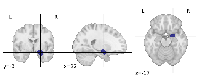
../../_images/053d022255c301a388229826c47d7ed67f910d4677ff4a126c073da57ffad942.png

Looks good! Now, finally, we can apply the ROI to our data in the same way we’d apply a mask: using the apply_mask function from Nilearn:

from nilearn import masking
R_ramyg = masking.apply_mask(R_4D, r_amygd_roi)
print("Shape of indexed data:", R_ramyg.shape)

Shape of indexed data: (40, 136)

Alright, that took some code, but we finally achieved what we wanted: a subset of voxels for our ROI (128 in total) for all our trials (40), neatly packaged in an $N \times K$ array!

ToDo (1 point): Repeat the ROI indexing process for our data (R_4D), but this time using an ROI of the left hippocampus. Store the results (a 2D array) in a variable named R_lhippocampus.

''' Implement your ToDo here. '''

# YOUR CODE HERE
raise NotImplementedError()

''' Tests the above ToDo. '''
assert(R_lhippocampus.shape == (40, 258))
print("Well done!")

PCA#

There are many methods for feature extraction, like “downsampling” to ROI-averages (i.e. averaging voxel patterns in brain regions) and dimensionality-reduction techniques like PCA. Scikit-learn provides some of these techniques as “transformer” objects, which again have a fit() and transform method. We’ll showcase this on the amygdala-restricted patterns we defined earlier.

from sklearn.decomposition import PCA
pca = PCA(n_components=10)

pca.fit(R_ramyg)
R_ramyg_pca10 = pca.transform(R_ramyg)
print("Shape after PCA:", R_ramyg_pca10.shape)

Shape after PCA: (40, 10)

ToDo (2 points): In the previous cell, we fitted the PCA to the entire dataset (all samples in R_ramyg), but again, ideally we'd add this a a step to our analysis pipeline and also cross-validate this procedure! Write a completely ) cross-validated decoding pipeline with 5 stratified folds that includes standardization (using RobustScaler), PCA dimenensionality reduction (using 10 components), and a logistic regression model which aims to predict expression (smiling vs. neutral). Keep track of the foldwise cross-validated accuracy on the test set and store the average accuracy in a variable named acc_av_todo.

''' Implement the ToDo here.'''

# YOUR CODE HERE
raise NotImplementedError()

''' Tests the above ToDo. '''
from niedu.tests.nipa.week_2 import test_pca_pipe    
test_pca_pipe(R_ramyg, S_expr, acc_av_todo)

Region averaging#

So far, we have restricted our analyses mostly to voxel patterns within a single ROI. For some research questions, however, you might want to include whole-brain patterns (for example, if you believe your experimental feature of interest is represented in whole-brain networks). This means, however, that you might be dealing with a lot of voxels (i.e., columns in your pattern matrix)! Again, you could reduce the number of features using dimensionality reduction techniques such as PCA. An alternative is to not use the activity of voxels as features, but the region-average activity! These regions can for example be derived from an existing anatomical atlas or parcellation or even from your own data (by fitting a clustering algorithm on the underlying timeseries).

You can do both (using existing atlases/parcellations or creating your own parcellation) using Nilearn. Here, we’ll demonstrate how to “downsample” your whole-brain voxel patterns to region-average patterns using the existing Shaefer et al. (2018) parcellation, which we can load in using Nilearn.

from nilearn.datasets import fetch_atlas_schaefer_2018
# It can return different number of ROIs; we'll set it to 100
schaefer_parc = fetch_atlas_schaefer_2018(n_rois=100, resolution_mm=2, verbose=False)

Note that the Schaefer parcellation is defined MNI space with a 2 millimeter resolution. Our data has the original BOLD resolution ($2.7 \times 2.7 \times 2.97$), so in order to use it on our data, we need to resample it:

# Set interpolation to nearest, because we're dealing with discrete integers
schaefer_rois = image.resample_to_img(schaefer_parc['maps'], R_4D, interpolation='nearest')

# Let's also plot it:
plotting.plot_roi(schaefer_rois);

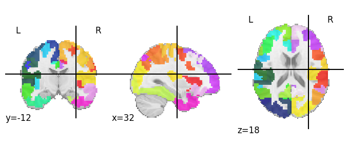
../../_images/589e89771bd7eed528c6bb5dbf3117684ff7cd15ae5f826b1a5f0bc4adb23f89.png

Note that, unlike the probabilistic ROIs that we used, the Schaefer parcellation is discrete: every voxel belongs to only a single region. As such, the ‘maps’ map in the schaef_parc object is a single volume with integers:

roi_ints = schaefer_rois.get_fdata()

# Let's check out the unique values in the volume
np.unique(roi_ints)

array([  0.,   1.,   2.,   3.,   4.,   5.,   6.,   7.,   8.,   9.,  10.,
        11.,  12.,  13.,  14.,  15.,  16.,  17.,  18.,  19.,  20.,  21.,
        22.,  23.,  24.,  25.,  26.,  27.,  28.,  29.,  30.,  31.,  32.,
        33.,  34.,  35.,  36.,  37.,  38.,  39.,  40.,  41.,  42.,  43.,
        44.,  45.,  46.,  47.,  48.,  49.,  50.,  51.,  52.,  53.,  54.,
        55.,  56.,  57.,  58.,  59.,  60.,  61.,  62.,  63.,  64.,  65.,
        66.,  67.,  68.,  69.,  70.,  71.,  72.,  73.,  74.,  75.,  76.,
        77.,  78.,  79.,  80.,  81.,  82.,  83.,  84.,  85.,  86.,  87.,
        88.,  89.,  90.,  91.,  92.,  93.,  94.,  95.,  96.,  97.,  98.,
        99., 100.])

Importantly, here, voxels with the value 0 represent background voxels (not belonging to any region). Now, using the NiftiLabelsMasker class from Nilearn, we can easly compute the ROI-average activity for each of our samples across the 100 ROIs in the Schaefer parcellation.

ToDo (1 point): Read through the documentation of the NiftiLabelsMasker class. Then, initialize a NiftiLabelsMasker object with labels_img=schaefer_rois and a "mean" strategy. Then, using this object, transform our whole-brain 4D patterns (the variable R_4D) into a 2D array (shape $40 \times 100$) and store it in a variable named R_schaefer.

''' Implement your ToDo here. '''
from nilearn.input_data import NiftiLabelsMasker

# YOUR CODE HERE
raise NotImplementedError()

''' Tests the above ToDo. '''    
from niedu.tests.nipa.week_2 import test_niftilabelsmasker
test_niftilabelsmasker(schaefer_rois, R_4D, R_schaefer)

Searchlight analysis#

One last technique that we want to discuss before moving on to statistical testing of decoding results is searchlight analysis (although it’s not really a feature selection/extraction technique). Searchlight analysis is a decoding-based analysis that is kind of a hybrid between univariate and multivariate analysis: it analyzes local voxel patterns but does that for every location in the brain. It does so by defining a spherical “searchlight” of voxels around a particular center voxel (with a particular radius). Within this searchlight, a (cross-validated) decoding analysis is performed and the result, usually a foldwise average model performance score (e.g., accuracy), is assigned to the center voxel. Then, the searchlight moved to the next voxel and a new decoding analysis performed; this process is repeated until each voxel has been the center voxel (and has been assigned a model performance score). As such, at the end of the searchlight analysis, you have an entire volume of (average) model performances, not just a single one!

Nilearn contains an efficient implementation of a searchlight analysis:

from nilearn.decoding import SearchLight

ToDo (0 points): Read through the documentation of the Searchlight estimator.

Just like other Nilearn (and scikit-learn) classes, we first need to initialize a Searchlight object. Upon initialization, the Searchlight class needs a couple of parameters:

mask_img: a binary mask that indicates which voxels contain actual brain;
process_mask_img: a binary mask that indicates which voxels should be analyzed;
radius: radius (in mm) of the searchlight sphere;
estimator: a scikit-learn compatible estimator (which can be a classifier/regression model or a Pipeline!)
n_jobs: how many CPUs to use
scoring: a string indicating which scoring method to (e.g., ‘accuracy’, ‘roc_auc’, etc.)
cv: either an integer (referring to the number of desired folds) or a cross-validation object (e.g., a StratifiedKFold object);
verbose: whether it should print out stuff while performing the fit (True or False)

Now, let’s go through these arguments one by one. First, to determine a brain mask, let’s just simply include all voxels that contain at least some signal across trials (i.e., where the sum across trials is not 0):

brain_mask = image.math_img('(img.sum(axis=3) != 0).astype(np.int32)', img=R_4D)
plotting.plot_roi(brain_mask);

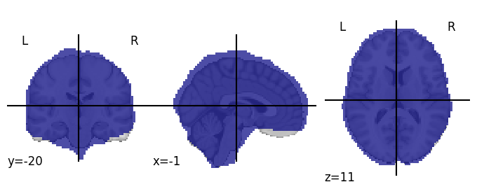
../../_images/b17f09fdd15d796a2802ffe6efe0d93a11fd762aacce1bb0a73dd8cac22c3255.png

ToThink (1 point): Why don't the inferior temporal lobes and the orbitofrontal cortex include any signal? Write your explanation in the text box below. Hint: think about the preprocessing tutorials from the previous course!

YOUR ANSWER HERE

For the process_mask_img, you could of course select the same mask (brain_mask), but for this tutorial, that would take too long. Instead, we’ll only analyze a single axial slice (the 22nd slice):

# Create empty volume
sl_mask = np.zeros(brain_mask.shape)

# Set the 22nd slice to 1
sl_mask[:, :, 21] = 1

# Create a Nifti1Image object from it using the "image.new_img_like" function
# from Nilearn
sl_mask = image.new_img_like(brain_mask, sl_mask)

# Of course, we only want to analyze the voxels from that slice that
# are ALSO in the brain mask, so let's intersect them:
sl_mask = masking.intersect_masks((brain_mask, sl_mask), threshold=1)

# Let's plot it:
plotting.plot_roi(sl_mask);

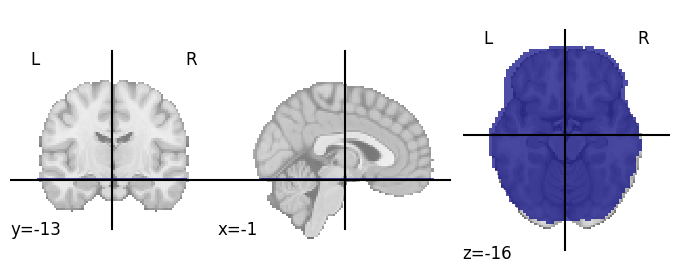
../../_images/141868cd2b0aaa15455bc72e082e20b2af0ae2495565ac000770e4c222acbd75.png

Lastly, we need to create an “estimator” and a cross-validation object. Let’s go for a simple pipeline with scaling and a LogisticRegression classifier and a StratifiedKFold CV scheme:

sl_cv = StratifiedKFold(n_splits=5, shuffle=True)
sl_estimator = make_pipeline(StandardScaler(), LogisticRegression(solver='lbfgs'))

Finally, we can initialize the Searchlight object:

sl = SearchLight(
    mask_img=brain_mask,
    process_mask_img=sl_mask,
    radius=5,  # we'll use a 5 mm radius
    estimator=sl_estimator,
    n_jobs=1,  # use only 1 core (for your own analyses, you might want to increase this!)
    scoring='roc_auc',  # use AUROC as model performance metric
    cv=sl_cv,
    verbose=True  # print a progressbar while fitting
);

To actually perform the searchlight analysis, we call the fit method with our data (a 4D nifti file, with the samples, $N$, in the fourth dimension) and target (the variable it needs to predict). The cell below might take a minute or two to run!

sl.fit(R_4D, S_expr);

After fitting, the Searchlight object’s scores_ attribute contains the voxelwise decoding scores (here: average AUROC scores across the five folds) as a 3D numpy array (with the same shape as our brain mask):

print("Shape scores_:", sl.scores_.shape)

Shape scores_: (73, 86, 66)

Let’s convert it to a Nifti1Image object so that we can plot it using Nilearn. We’ll set the (somewhat arbitrarily chosen) threshold to 0.65:

score_img = image.new_img_like(brain_mask, sl.scores_)
plotting.plot_stat_map(score_img, threshold=0.65);

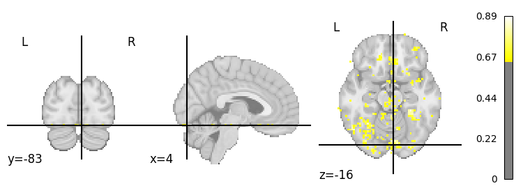
../../_images/1d9aa8d3dffd7d5b18ff817ceabe13bc3dd09d249758e411d62a5bc49abac0dc.png

If you want to know more about searchlight analyses, we recommend this article. That said, let’s continue with the last part of this tutorial: permutation testing!

Significance tests and permutation testing#

Suppose you ran your decode pipeline on twenty subjects and accordingly collected a set of twenty model performance scores (e.g., accuracy for a two-class target). Inevitably, some scores will be higher (e.g., 0.9) than others (e.g., 0.7), and some may even be at or below chance level (e.g., 0.45). In the same vein, suppose you ran your decode pipeline across the gray-matter density patterns of a 100 subjects (of which 50 are diagnosed with major depression and 50 are healthy controls) in a 10-fold cross-validation scheme, yielding tne (foldwise) model performance scores. Again, the magnitude of these scores may differ. How do we determine if these scores are, in fact, significantly higher than we’d expect by chance?

Significance tests for within-subject decoding analyses can be done in two ways. The “easy” way is to simply do a one-sample $t$-test against chance-level (e.g., 0.5 for a two-class target) on the subject-wise model performance scores. For example, suppose that our analyses have produced the following model performance scores (e.g., accuracy, averaged across folds):

# acc_scores are the average (across folds) accuracy score
acc_scores = np.array([0.5, 0.65, 0.55, 0.7, 0.85, 0.65, 0.9, 0.45, 0.55, 0.50])

As it is reasonable to assume that subjects are independent, we can do a one-sample $t$-test against a $H_{0}$ of 0.5:

from scipy.stats import ttest_1samp
tvalue, pvalue = ttest_1samp(acc_scores, popmean=0.5)
print("T-value: %.3f, p-value: %.3f" % (tvalue, pvalue))

T-value: 2.717, p-value: 0.024

If we’d use a significance level ($\alpha$) of 0.05, this would mean that our result is statistically significant — yay! This simple approach is, however, technically not a completely valid (random effects) analysis as shown by Allefeld and colleagues (2016), because a one-sample t-test assumes a symmetric distribution centered at chance-level, but below chance-level model performance in the population is impossible. This is like testing commute time of people against a null-hypothesis of 0, which doesn’t make sense, because you cannot have a negative commute time! Allefeld and colleagues propose a solution, which they call “prevalence inference”, which involves intricate permutation testing procedures and is a bit too complicated for this course. If you ever need to evaluate decoding performance at the group-level, though, we highly recommend trying to implement this method.

Tip: If you want to know more about prevalence inference and want to see some example code, you can check out this notebook.

That said, let’s look at how we’d statistically test the results of between-subject analyses. We cannot use a simple one-sample $t$-test for between-subject results, because data points in between-subject analyses — usually the model performance scores associated with different folds in K-fold CV — are not independent, which is an important assumption of all parametric statistics (such as $t$-tests). Dependence between data points is created because the same samples may be included in different folds. As such, we need a different, non-parameteric approach to evaluate statistical significance: permutation testing.

In the previous sections of this tutorial, we worked with within-subject data from a single subject, but for this section, we’ll need some between-subject data. For this, we’ll use voxel-based morphometry (VBM) data from 47 subjects. We’ll use these voxelwise gray matter volume patterns in the bilateral caudate to predict subject gender (male vs. female). Although theoretically meaningless, this allows us to demonstrate permutation testing.

First, let’s load in and prepare the data:

with open('vbm_analysis_data.npz', 'rb') as f_in:
    data = np.load(f_in)
    R, S = data['R'], data['S']

print("R shape:", R.shape)
print("S shape:", S.shape)

R shape: (47, 901)
S shape: (47,)

As you can see, we have data from 47 subjects with 901 voxels from the bilateral caudate.

Getting your observed performance score#

Before you start with anything related to permutation testing, you first need to get your performance score that you would like to get a $p$-values for. In between-subject decoding analyses, this is usually the average accuracy (or whatever other metric) across folds. So, when you would implement a 3-fold cross-validation scheme, your observed performance score would be the average of the accuracy-estimates across those 3 folds. You know what? Let’s implement exactly that:

pipe = make_pipeline(StandardScaler(), LogisticRegression(solver='lbfgs', class_weight='balanced'))

np.random.seed(42)  # for reproducibility

# We'll pick 3 folds
skf = StratifiedKFold(n_splits=3)

performance = []
for train_idx, test_idx in skf.split(R, S):
    R_train, R_test = R[train_idx, :], R[test_idx, :]
    S_train, S_test = S[train_idx], S[test_idx]
    
    pipe.fit(R_train, S_train)
    preds = pipe.predict(R_test)
    performance.append(accuracy_score(S_test, preds))
    
observed_acc = np.mean(performance)
print("Mean accuracy across folds = %.3f" % observed_acc)

Mean accuracy across folds = 0.636

Alright, not bad! 63.6% correct is higher than chance, but is it also significantly higher than chance? For that, we need to “simulate” a null-distribution through permutation!

Getting your permuted performance distribution#

The goal of permutation tests are to create a null-distribution of your observed measure, in this case: (average) classification accuracy. The null-distribution refers to the distribution of classification accuracies that would arise if you would repeat an experiment with noisy data in which there is no effect (i.e. the null-hypothesis is true).

Thus, we need to somehow repeat the above “experiment” (i.e. the analysis which yielded the observed performance of 51.1%) yet while the null-hypothesis is true (i.e. there is no effect, only noise). Well, as the term “permutation” suggest, we can simply randomly shuffly the train-labels (S_train) to generate random labels. Now, if we would fit the classifier on {R_train, and S_train}, then practically it would fit on noise. In fact, by random shuffling of the train-labels, we simulated the scenario in which (on average) the null-hypothesis would be true.

So, what we need to do in order to create a null-distribution of classification-accuracies is to run our original analysis (in the code cell above) many times (i.e. “repeat the experiment”), yet with random labeling of our train-samples. We expect that the mean of these null-accuracies would center around .5 (assumed chance level), but simply due to random noise, our simulated null-distribution will contain values (sometimes substantially) above and below chance level.

Anyway, look at the code-cell below. It contains exactly the same analysis as in the above code-block, yet now it is looped 100 times, and just before fitting (within every fold separately) we shuffle the train-labels to generate a random mapping between R_train and S_train. After every “experiment” (or simply “permutation”) we average the permuted accuracy scores across folds and store them (in the variable permuted_accuracies). Now, let’s run the code cell below (may take minute or two):

from tqdm import tqdm

n_permutations = 100
permuted_accuracies = np.zeros(n_permutations)

# the tqdm thingie will print a nice progressbar below
for i in tqdm(range(n_permutations)):

    folds = skf.split(R, S)
    fold_accuracies = np.zeros(skf.get_n_splits())

    for ii, (train_idx, test_idx) in enumerate(folds):
    
        X_train, X_test = R[train_idx], R[test_idx]
        y_train, y_test = S[train_idx], S[test_idx]
    
        # Here we shuffle the S-train labels!!!
        np.random.shuffle(S_train)
        
        pipe.fit(R_train, S_train)
        preds = pipe.predict(R_test)
        fold_accuracies[ii] = accuracy_score(S_test, preds)
    
    permuted_accuracies[i] = np.mean(fold_accuracies)

Okay, we now got our simulated null-distribution values stored in the variable permuted_accuracies. Let’s look at how the distribution actually looks like (and how the observed accuracy relates to the permuted scores):

import matplotlib.pyplot as plt

plt.figure(figsize=(10, 5))
plt.title('Permuted null-distribution')
plt.hist(permuted_accuracies)
plt.xlabel('Average accuracy across folds')
plt.ylabel('Frequency')
plt.axvline(observed_acc, c='r', ls='--')
plt.legend(['Observed score'], frameon=False)
plt.show()

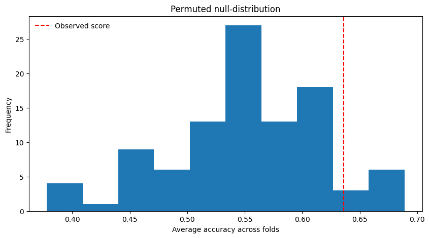
../../_images/8162fed2bee31110e1c2599262b4b2ffd849e6160cde6b598dcca30745fd21d5.png

Now, the ‘formula’ for the $p$-value in a permutation test is as follows: given $P$ permutations, it’s the following (in pseudo-notation):

(98)#\[\begin{align} p = \frac{\sum_{i=1}^{P}{(\mathrm{permuted}_{i} \geq \mathrm{observed})} + 1}{P+1} \end{align}\]

where $(\mathrm{permuted}_{i} \geq \mathrm{observed})$ evaluates to 1 if true, otherwise 0. Put differently: the $p$-value, here, expresses the proportion of permutation-values that is equal to or higher than the observed value. Graphically, we can visualize the $p$-value as the area of the (simulated!) null-distribution right of the dotted red line in the figure above.

ToDo (1 point): Calculate the $p$-value corresponding to the observed accuracy given our permuted null-distribution. Store it in a variable named pval_permutation.

# calculate p-value

# YOUR CODE HERE
raise NotImplementedError()

''' Tests the above ToDo.'''
from niedu.tests.nipa.week_2 import test_perm_pval
test_perm_pval(permuted_accuracies, observed_acc, pval_permutation)

ToDo (2 points): For this final ToDo, we are going to throw you in at the deep end. Instead of a classification analysis, you are going to implement a regression analysis, in which you'll try to predict 'average attractiveness' (i.e., the attractiveness ratings for our stimuli given by an external set of subjects), which we defined for you already (the variable S, below). For the patterns, you can reuse the R_4D variable. However, you need to index this with a "Frontal Orbital Cortex" ROI from the Harvard-Oxford atlas (also defined below: ho_atlas). Note, you have to define the ROI yourself (including resampling to match the resolution of the patterns).

Then, construct a pipeline with a StandardScaler and a Ridge regression model (from the linear_model module; do not use any specific arguments during initialization). Using a 4-fold cross-validation routine (using the KFold class from the model_selection module), compute the cross-validated mean squared error (either manually or using the mean_squared_error function from the metrics module) each iteration. Finally, average the four mean squared error values and store this in a variable named av_mse.

A couple of pointers:

You need to import all (new) classes and functions yourself;
Realize that scikit-learn uses a consistent interface for its classes, whether they are regression-related or classification-related (e.g., a regression model has largely the same methods as classification models);

Good luck!

''' Implement your ToDo here. '''
S = events['average_attractiveness'].values
ho_atlas = fetch_atlas_harvard_oxford('cort-maxprob-thr50-2mm')

np.random.seed(42)

# YOUR CODE HERE
raise NotImplementedError()

''' Tests the above ToDo. '''
from niedu.tests.nipa.week_2 import test_regression_todo
test_regression_todo(R_4D, events, av_mse)

This notebook discussed the basics of decoding analyses. There are many more topics that we didn’t discuss (such as regularization, hyperparameter optimalization, prevalence inference), but hopefully you can get started with implementing your own decoding analyses after having completed this notebook!

Machine learning (“decoding”) analyses

Contents

Machine learning (“decoding”) analyses#

Data representation#

Standardization#

Fitting models#

Model evaluation#

Metrics for discrete predictions#

Metrics for probabilistic predictions#

Cross-validation#

Train vs. test set partitioning#

Sidenote: scikit-learn Pipelines#

Class imbalance and model performance revisited#

Feature selection/extraction#

ROI selection#

PCA#

Region averaging#

Searchlight analysis#

Significance tests and permutation testing#

Getting your observed performance score#

Getting your permuted performance distribution#

Sidenote: scikit-learn `Pipelines`#