
An introduction to Nilearn#
This notebook is about the amazing nilearn Python package for applying statistical learning techniques (from GLMs to multivariate “decoding” and connectivity techniques) to neuroimaging data. In addition, it features all kinds of neat functionality like automic fetching of publicly available data, (interactive) visualization of brain images, and easy image operations.
In this tutorial, we’ll walk you through the basics of the package’s functionality in a step-by-step fashion. Notably, this notebook contains several exercises (which we call “ToDos”), which are meant to make this tutorial more interactive! Also, this tutorial is merely an introduction to (parts of) the Nilearn package. We strongly recommend checking out the excellent user guide and example gallery on the Nilearn website if you want to delve deeper into the package’s (more advanced) features.
Contents
What is Nilearn?
Data formats
Data visualization
Image manipulation
Region extraction
Connectome/connectivity analyses
Estimated time needed to complete: 1-3 hours (depending on your experience with Python)
Credits: if you end up using nilearn in your work, please cite the corresponding article.
# Let's see whether Nilearn is installed
try:
import nilearn
except ImportError:
# if not, install it using pip
!pip install nilearn
What is Nilearn?#
Nilearn is one of the packages in the growing “nipy” ecosystem of Python packages for neuroimaging analysis (see also MNE, nistats, nipype, nibabel, and dipy). Specifically, Nilearn provides tools for analysis techniques like functional connectivity, multivariate (machine-learning based) “decoding”, but also more “basic” tools like image manipulation and visualization.
On Nilearn’s website, you can see that the package contains several modules (such as connectome, datasets, decoding, etc.). In the following sections, we will discuss some of them.
Data formats#
Nilearn’s functionality assumes that your MRI data is stored in nifti images. Many functions in Nilearn accept either strings pointing towards the path of a nifti file (or a list with multiple paths) or a Nifti1Image object from the nibabel package. Together, these two types of inputs (filenames pointing to nifti files and nibabel Nifti1Images) are often referred to a “niimgs” (or “niimg-like”) by Nilearn — a term you’ll see a lot in Nilearn’s documentation (for more info about data formats in Nilearn, see this explainer).
Before we go on, let’s actually download some example nifti files to work with. Fortunately, Nilearn has an entire module dedicated to fetching example data and other useful files (e.g., atlases): nilearn.datasets. We’ll import it below:
from nilearn import datasets
Now, we will download some example data from the famous Haxby et al. (2001) study. This can be done using the fetch_haxy function from the datasets module. We’ll download data from only a single subject for now.
# This might take a while, depending on your internet speed
data = datasets.fetch_haxby(
data_dir=None,
subjects=1,
fetch_stimuli=False,
verbose=1
)
Dataset created in /home/runner/nilearn_data/haxby2001
Downloading data from https://www.nitrc.org/frs/download.php/7868/mask.nii.gz ...
Downloading data from http://data.pymvpa.org/datasets/haxby2001/MD5SUMS ...
Downloading data from http://data.pymvpa.org/datasets/haxby2001/subj1-2010.01.14.tar.gz ...
The fetch_haxby function returns a dictionary with the location of the downloaded files and some metadata:
from pprint import pprint # useful function to "pretty print" dictionaries
pprint(data)
{'anat': ['/home/runner/nilearn_data/haxby2001/subj1/anat.nii.gz'],
'description': 'Haxby 2001 results\n'
'\n'
'\n'
'Notes\n'
'-----\n'
'Results from a classical fMRI study that investigated the '
'differences between\n'
'the neural correlates of face versus object processing in the '
'ventral visual\n'
'stream. Face and object stimuli showed widely distributed and '
'overlapping\n'
'response patterns.\n'
'\n'
'Content\n'
'-------\n'
'The "simple" dataset includes\n'
" :'func': Nifti images with bold data\n"
" :'session_target': Text file containing session data\n"
" :'mask': Nifti images with employed mask\n"
" :'session': Text file with condition labels\n"
'\n'
'\n'
'The full dataset additionally includes\n'
" :'anat': Nifti images with anatomical image\n"
" :'func': Nifti images with bold data\n"
" :'mask_vt': Nifti images with mask for ventral "
'visual/temporal cortex\n'
" :'mask_face': Nifti images with face-reponsive brain "
'regions\n'
" :'mask_house': Nifti images with house-reponsive brain "
'regions\n'
" :'mask_face_little': Spatially more constrained version "
'of the above\n'
" :'mask_house_little': Spatially more constrained version "
'of the above\n'
'\n'
'\n'
'References\n'
'----------\n'
'For more information see:\n'
'PyMVPA provides a tutorial using this dataset :\n'
'http://www.pymvpa.org/tutorial.html\n'
'\n'
'More information about its structure :\n'
'http://dev.pymvpa.org/datadb/haxby2001.html\n'
'\n'
'\n'
'`Haxby, J., Gobbini, M., Furey, M., Ishai, A., Schouten, J.,\n'
'and Pietrini, P. (2001). Distributed and overlapping '
'representations of\n'
'faces and objects in ventral temporal cortex. Science 293, '
'2425-2430.`\n'
'\n'
'\n'
'Licence: unknown.\n',
'func': ['/home/runner/nilearn_data/haxby2001/subj1/bold.nii.gz'],
'mask': '/home/runner/nilearn_data/haxby2001/mask.nii.gz',
'mask_face': ['/home/runner/nilearn_data/haxby2001/subj1/mask8b_face_vt.nii.gz'],
'mask_face_little': ['/home/runner/nilearn_data/haxby2001/subj1/mask8_face_vt.nii.gz'],
'mask_house': ['/home/runner/nilearn_data/haxby2001/subj1/mask8b_house_vt.nii.gz'],
'mask_house_little': ['/home/runner/nilearn_data/haxby2001/subj1/mask8_house_vt.nii.gz'],
'mask_vt': ['/home/runner/nilearn_data/haxby2001/subj1/mask4_vt.nii.gz'],
'session_target': ['/home/runner/nilearn_data/haxby2001/subj1/labels.txt']}
Let’s inspect the "description" in more detail, which described the contents of the dictionary:
print(data['description'])
Haxby 2001 results
Notes
-----
Results from a classical fMRI study that investigated the differences between
the neural correlates of face versus object processing in the ventral visual
stream. Face and object stimuli showed widely distributed and overlapping
response patterns.
Content
-------
The "simple" dataset includes
:'func': Nifti images with bold data
:'session_target': Text file containing session data
:'mask': Nifti images with employed mask
:'session': Text file with condition labels
The full dataset additionally includes
:'anat': Nifti images with anatomical image
:'func': Nifti images with bold data
:'mask_vt': Nifti images with mask for ventral visual/temporal cortex
:'mask_face': Nifti images with face-reponsive brain regions
:'mask_house': Nifti images with house-reponsive brain regions
:'mask_face_little': Spatially more constrained version of the above
:'mask_house_little': Spatially more constrained version of the above
References
----------
For more information see:
PyMVPA provides a tutorial using this dataset :
http://www.pymvpa.org/tutorial.html
More information about its structure :
http://dev.pymvpa.org/datadb/haxby2001.html
`Haxby, J., Gobbini, M., Furey, M., Ishai, A., Schouten, J.,
and Pietrini, P. (2001). Distributed and overlapping representations of
faces and objects in ventral temporal cortex. Science 293, 2425-2430.`
Licence: unknown.
Alright, now we have some data to work with. With the image module in Nilearn, we can load in and perform many different operations on nifti images. We’ll import it below:
from nilearn import image
And let’s load in the anatomical image from the Haxby dataset that we downloaded using the load_img function from the image module:
anat_img = image.load_img(data['anat'])
print("The variable anat_img is an instance of the %s class!" % type(anat_img).__name__)
The variable anat_img is an instance of the Nifti1Image class!
Note that load_img is basically the same as the nibabel function load, but with some extra functionality (like loading in a list of files using wildcards) and checks (like whether it’s really a nifti image).
Also, note that the anat_img is an object instantiated from the custom Nifti1Image class.
print(type(anat_img))
<class 'nibabel.nifti1.Nifti1Image'>
# Try it below!
# YOUR CODE HERE
raise NotImplementedError()
''' Tests the ToDo above. '''
# Check shape (should be 5 volumes)
assert(all_mask_imgs.shape == (40, 64, 64, 5))
print("Well done!")
In general, Nilearn contains several functions that can be seen as “wrappers” around common operations that you’d normally use nibabel and/or numpy for, such as creating new Nifti images from numpy arrays (image.new_img_like), indexing (4D) images (image.index_img), and averaging 4D images across time (image.mean_img). For example, suppose we have a 3D numpy array containing, e.g., \(\hat{\beta}\) values from a GLM analysis with the same shape as our anatomical scan:
import numpy as np
arr_3d = np.random.normal(0, 1, size=anat_img.shape)
print("The variable arr_3d is an instance of the %s class!" % type(arr_3d).__name__)
The variable arr_3d is an instance of the ndarray class!
Now, suppose we want to convert this data to a nibabel Nifti1Image object, so that we can perform other operations on it or visualize it (using Nilearn). We can use the new_img_like function for this:
arr_3d_img = image.new_img_like(ref_niimg=anat_img, data=arr_3d)
print("The variable arr_3d_img is an instance of the %s class!" % type(arr_3d_img).__name__)
The variable arr_3d_img is an instance of the Nifti1Image class!
Before we go into more detail, let’s make it a little bit more interesting by focusing on the data visualization tools within Nilearn.
Data visualization#
The data visualization tools in Nilearn are grouped in the plotting module. The plotting module, in our opinion, is one of Nilearn’s most useful features!
Alright, let’s start by importing the module (and telling Jupyter to plot our figures inside the notebook using %matplotlib inline):
from nilearn import plotting
%matplotlib inline
We can try plotting our anat_img (high-resolution T1-weighted image) using the plot_anat function. In the most basic approach, you can simply call it with your image (a Nifti1Image or path to a nifti file) as the first argument:
display = plotting.plot_anat(anat_img)
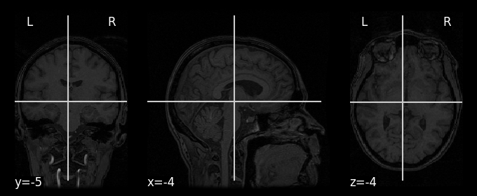
Note that the variable display is an instance of a custom Nilearn class (Orthoslicer) which contains some nifty (pun intended) features as well (which we won’t discuss here, but check out Nilearn’s plotting reference).
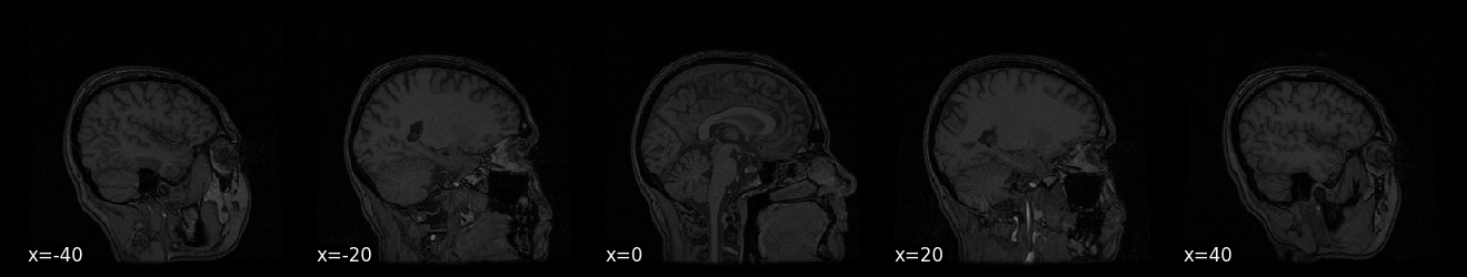
But Nilearn plotting functions contain many (optional) arguments that you can use to customize your plot. For example, the display_mode argument allows you to plot the image in one (or more) particular dimensions (e.g., the “X” axis, which is usually sagittal) and the cut_coords argument allows you to specify the number (if integer) or locations of the particular slices/cuts (if list):
display = plotting.plot_anat(anat_img, display_mode='x', cut_coords=[-40, -20, 0, 20, 40])
# Implement your ToDo here
# YOUR CODE HERE
raise NotImplementedError()
There are many other plotting functions besides plot_anat, which we’ll highlight when relevant in the next sections of this tutorial.
Image manipulation#
Nilearn contains a lot of functionality to easily manipulate images. Note that, again, all of this could be implemented with numpy (in fact, Nilearn uses numpy “under the hood” for many of its operations); just see the Nilearn functions as “wrappers” around common numpy routines for nifti-based arrays (which also handle the updating of image affines, e.g. after resampling an image, appropriately).
To showcase some nilearn functions, we’ll use the functional MRI data we downloaded (bold.nii.gz).
func_img = image.load_img(data['func'][0])
print("Shape of functional MRI image: %s" % (func_img.shape,))
Shape of functional MRI image: (40, 64, 64, 1452)
This file, however, is quite large (~400 MB), as it contains concatenated data across 12 runs. To limit the amount of data that we need to load into RAM, we’ll only load in the data from the first run. We can find out which volumes belong to which run in the “session_target” information, which we’ll load in below as a pandas dataframe:
import pandas as pd
metadata = pd.read_csv(data['session_target'][0], sep=' ')
print("Shape of metadata dataframe: %s" % (metadata.shape,), end='\n\n')
metadata.head(20)
Shape of metadata dataframe: (1452, 2)
| labels | chunks | |
|---|---|---|
| 0 | rest | 0 |
| 1 | rest | 0 |
| 2 | rest | 0 |
| 3 | rest | 0 |
| 4 | rest | 0 |
| 5 | rest | 0 |
| 6 | scissors | 0 |
| 7 | scissors | 0 |
| 8 | scissors | 0 |
| 9 | scissors | 0 |
| 10 | scissors | 0 |
| 11 | scissors | 0 |
| 12 | scissors | 0 |
| 13 | scissors | 0 |
| 14 | scissors | 0 |
| 15 | rest | 0 |
| 16 | rest | 0 |
| 17 | rest | 0 |
| 18 | rest | 0 |
| 19 | rest | 0 |
Here, “chunks” refer to the specific run index and “labels” refers to the timepoint-by-timepoint condition (i.e., the condition of the active block at each moment in time, e.g., images of scissors, images of chairs, rest blocks, etc.). Let’s compute the number of timepoints in the first “chunk” (run):
nvol_run_1 = np.sum(metadata['chunks'] == 0)
print("Number of volumes in run 1: %i" % nvol_run_1)
Number of volumes in run 1: 121
Alright, now we can use Nilearn’s index_img function from the image module to index our func_img object.
to_index = np.arange(nvol_run_1, dtype=int)
func_img_run1 = image.index_img(func_img, to_index)
print("Shape of func_img_run1: %s" % (func_img_run1.shape,))
Shape of func_img_run1: (40, 64, 64, 121)
# Implement the ToDo here
# YOUR CODE HERE
raise NotImplementedError()
''' Tests the above ToDo. '''
assert(length_run1 == 302.5)
Okay, that was the boring part. Let’s do some more interesting things!
Image mathematics#
Nilearn provides some functions to make your life easier when doing array mathematics on 3D or 4D images. For example, the mean_func from the image module computes the mean across time for every voxel in a 4D image. (Note that, again, this could also be done in numpy.)
# Implement the ToDo here.
# YOUR CODE HERE
raise NotImplementedError()
''' Tests the above ToDo. '''
assert(mean_func.shape == (40, 64, 64))
print("Well done!")
# YOUR CODE HERE
raise NotImplementedError()
Another useful function from the image module is math_img. This function allows you to perform more complex mathematical operations to entire images at once. For example, suppose you want to mean-center the time series of every voxel \(v\) in an image (i.e., subtract the mean across time from each time point).
We can do that as follows using math_img:
mean_centered_img = image.math_img('img - np.mean(img, axis=3, keepdims=True)', img=func_img_run1)
As you can see, the function math_img takes a string indicating a particular (numpy) operation on the variable “img”, which is given as an argument to the function. You can give as many extra arguments (associated with particular images) to the function as you’d like. For example, the above operation can also be performed as follows:
# Recompute mean_func because of ToDo
mean_func = image.mean_img(func_img_run1)
mean_centered_img = image.math_img('img_4d - img_mean[:, :, :, np.newaxis]', img_4d=func_img_run1, img_mean=mean_func)
# Implement the ToDo here
# YOUR CODE HERE
raise NotImplementedError()
''' Tests the above ToDo. '''
np.testing.assert_almost_equal(
tsnr_func.get_fdata()[20, 30, 30],
64.76949,
decimal=5
)
print("Well done!")
Image preprocessing#
Nilearn also provides some functionality for basic preprocessing of (functional) images. Note the adjective “basic” — most preprocessing steps (such as image registration, motion correction, susceptibility distortion correction, etc.) should be done using other packages (for which we strongly recommend Fmriprep). That said, Nilearn does provide some preprocessing functionality, such as smoothing (with image.smooth_img):
# Recompute tsnr_func because of ToDo
tsnr_func = image.math_img('img.mean(axis=3) / img.std(axis=3)', img=func_img_run1)
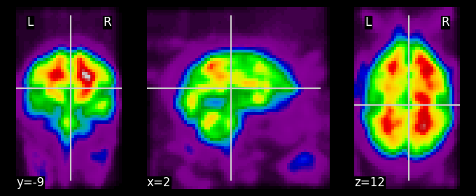
tsnr_func_smooth = image.smooth_img(tsnr_func, fwhm=10)
display = plotting.plot_epi(tsnr_func_smooth);
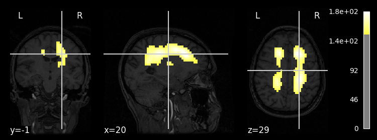
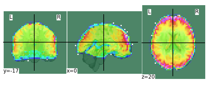
Hmm, perhaps it would be nicer to plot a thresholded version of this map on the subject’s high-resolution T1-weighted scan … Of course, Nilearn has a function for that: plot_stat_map, which takes both a “stat_map” (which can be anything, as long as it’s a 3D image) and a background image, as well as an optional threshold argument:
display = plotting.plot_stat_map(tsnr_func_smooth, bg_img=anat_img, threshold=150)
Note that you can even create interactive image viewers using, for example, the view_img function. This works especially well in Jupyter notebooks. Importantly (at least in Jupyter notebooks), you should call this plotting function at the end of the code cell and you should not assign the output of the function to a new variable, otherwise the viewer won’t render.
# Do not add code after this line, otherwise it won't work
plotting.view_img(tsnr_func_smooth, bg_img=anat_img, threshold=150)
While these interactive viewers are amazing, be careful not to open too many of them, as they need quite a bit of memory to run!
Don’t forget to import the masking module!
# Implement your ToDo here
# YOUR CODE HERE
raise NotImplementedError()
''' Tests the above ToDo. '''
assert(func_mask.get_fdata().sum() == 23594)
print("Well done!")
In addition to spatial smoothing and creating (functional) brain masks, Nilearn actually also provides some tools for preprocessing in the time domain (such as detrending,
Image masking#
A common operation in fMRI analyses is masking: extracting particular voxels from the entire dataset, usually based on a binary brain mask (like you computed in the previous ToDo). Masking, at least in fMRI analyses, is often done on the spatial dimensions of 4D images; as such, masking can be seen as a operation that takes in a 4D image with spatial dimensions \(X \times Y \times Z\) and temporal dimension \(T\) and returns a \(T \times K\) 2D array, where \(K\) is the number of voxels that “survived” (for lack of a better word) the masking procedure.
Reasons to mask your data could be, for example, to exclude non-brain voxels (like in skullstripping) or to perform confirmatory region-of-interest (ROI) analyses, or to extract one or multiple “seed regions” for connectivity analyses.
Nilearn provides several functions and classes that perform masking, which differ in how extensive they are (some only perform masking on a single image, others do this for multiple images at the same time, and/or may additionally perform preprocessing steps). Importantly, all take in a 4D niimg-like object and return a 2D numpy array.
We’ll first take a look at the most simple and low-level implementation: apply_mask. This function takes in a 4D image (which will be masked), a binary 3D image (i.e., with only zeros and ones, where ones indicate that they should be included) as mask, and optionally a smoothing kernel size (FWHM in millimeters) and returns a masked 2D array. Let’s do this for our data (func_img_run1) using the brain mask (func_mask) you computed earlier:
from nilearn import masking
# Let's compute the epi mask again, in case you didn't do this in the previous ToDo
func_mask = masking.compute_epi_mask(mean_func)
print("Before masking, our data has shape %s ..." % (func_img_run1.shape,))
func_masked = masking.apply_mask(func_img_run1, func_mask)
print("... and afterwards our data has shape %s and is a %s" % (func_masked.shape, type(func_masked).__name__))
Before masking, our data has shape (40, 64, 64, 121) ...
... and afterwards our data has shape (121, 23594) and is a ndarray
Importantly, we can “undo” the masking operation by the complementary unmask function:
func_unmasked = masking.unmask(func_masked, func_mask)
print("func_unmasked is a %s and has shape %s" % (type(func_unmasked).__name__, func_unmasked.shape))
func_unmasked is a Nifti1Image and has shape (40, 64, 64, 121)
# Implement your ToDo here
# YOUR CODE HERE
raise NotImplementedError()
'''Tests the above ToDo. '''
tmp_test = tsnr_masked_img.get_fdata()
np.testing.assert_array_equal(
tmp_test[30, 30, 30, :5],
np.array([1695., 1712., 1690., 1695., 1711.])
)
np.testing.assert_array_equal(
tmp_test[20, 30, 30, :],
np.zeros(tmp_test.shape[-1])
)
print('Well done!')
Apart from the apply_mask and unmask functions, Nilearn also contains a more extensive “masking” class, NiftiMasker (from the input_data module), that has some extra preprocessing features. Unlike the name suggests, this class does much more than masking: it also (optionally) allows you to spatially and temporally preprocess your data! It works slightly differently than the relatively simple functions we have discussed so far though, so we’ll spend a little time on its “mechanics”.
We’ll start with importing it:
from nilearn.input_data import NiftiMasker
Importantly, NiftiMasker is not a function, but a (custom) class. With this class, you can create (or “initialize”) a new object of this class. Upon inialization, you can give it particular arguments that define how the NiftiMasker object will behave. Read through the documentation of the NiftiMasker class to see which arguments it accepts.
For now, we’ll initialize a very simple NiftiMasker that only accepts a particular brain mask (and set verbose=True to print some extra information).
masker = NiftiMasker(mask_img=func_mask, verbose=True)
print("The masker variable is a %s object" % type(masker).__name__)
The masker variable is a NiftiMasker object
Realize that we haven’t masked anything, yet! We can do this using the fit and transform methods of NiftiMasker objects. This “design” (i.e., custom objects with fit and transform methods that implement data transformations) is based on the design principles of the scikit-learn Python package for machine learning (some of the authors of the Nilearn package also created and contribute to the scikit-learn package).
Now, after initialization of the NiftiMasker object, you need to call the fit method, which needs the to-be-transformed (here: masked) 4D image as an input:
masker.fit(func_img_run1)
[NiftiMasker.fit] Loading data from Nifti1Image(
shape=(40, 64, 64, 121),
affine=array([[ -3.5 , 0. , 0. , 68.25 ],
[ 0. , 3.75 , 0. , -118.125],
[ 0. , 0. , 3.75 , -118.125],
[ 0. , 0. , 0. , 1. ]])
)
[NiftiMasker.fit] Resampling mask
NiftiMasker(mask_img=<nibabel.nifti1.Nifti1Image object at 0x7f53eadfd280>,
verbose=True)In a Jupyter environment, please rerun this cell to show the HTML representation or trust the notebook. On GitHub, the HTML representation is unable to render, please try loading this page with nbviewer.org.
NiftiMasker(mask_img=<nibabel.nifti1.Nifti1Image object at 0x7f53eadfd280>,
verbose=True)In the output block of the cell above (Out[xx]), you can see that the fit function returns “itself” (i.e., the NiftiMasker object). Importantly, any computations are happening “in-place”, so the output (i.e., the object itself) does not need to be stored in a new variable.
Moreover, because we set verbose=True, some extra information about what the NiftiMasker does is printed (first, the data from func_img_run1 is loaded in memory and, second, the func_mask is resampled to the same space as the func_img_run1 if necessary).
Again, even after calling fit, our 4D data not been masked yet! The fitting procedure only makes sure that the NiftiMasker object is ready to transform whatever image you want (later, when you call transform). You might think, “why do you need a fit method, if it is not actually ‘fitting’ anything?” In this example, it is indeed redundant, but there are many other features in the NiftiMasker class that actually perform some computation. For example, we could initialize a NiftiMasker object without an explicit mask_img, but with the argument mask_strategy='epi', which will actually compute a functional brain mask when you will call fit:
masker2 = NiftiMasker(mask_strategy='epi', verbose=1)
masker2.fit(func_img_run1);
[NiftiMasker.fit] Loading data from Nifti1Image(
shape=(40, 64, 64, 121),
affine=array([[ -3.5 , 0. , 0. , 68.25 ],
[ 0. , 3.75 , 0. , -118.125],
[ 0. , 0. , 3.75 , -118.125],
[ 0. , 0. , 0. , 1. ]])
)
[NiftiMasker.fit] Computing the mask
[NiftiMasker.fit] Resampling mask
Here, you see that the computation of the mask is happening when we called fit. In general, this design pattern — which defers any computation to a particular method (here: fit) and uses a different method (e.g., transform) for the actual transformation — is ideal for cross-validation. Cross-validation is a procedure where you want to use separate subsets of your data for estimating (fitting) parameters or operations and actually applying those parameters or operations, which is common in, for example, machine learning.
Anyway, we are digressing. After calling fit, we can now call the transform method with the image that we want to transform (here: mask) as input, which will return the masked image:
# would be the same for the masker2 object
masked_file = masker.transform(func_img_run1)
print("\nThe variable masked_file is an instance of the %s class," % type(masked_file).__name__)
print("with shape %s" % (masked_file.shape,))
[NiftiMasker.transform_single_imgs] Loading data from Nifti1Image(
shape=(40, 64, 64, 121),
affine=array([[ -3.5 , 0. , 0. , 68.25 ],
[ 0. , 3.75 , 0. , -118.125],
[ 0. , 0. , 3.75 , -118.125],
[ 0. , 0. , 0. , 1. ]])
)
[NiftiMasker.transform_single_imgs] Extracting region signals
[NiftiMasker.transform_single_imgs] Cleaning extracted signals
The variable masked_file is an instance of the ndarray class,
with shape (121, 23594)
Note that transform again need the to-be-transformed image (here: func_img_run1) as input, but this could have been any other 4D image (as long as it has the same dimensions)!
To make your life a little easier, NiftiMasker objects also contain another function, fit_transform, that (guess what) combines the fit and transform methods in a single method:
masked_file = masker.fit_transform(func_img_run1)
[NiftiMasker.fit] Loading data from None
[NiftiMasker.fit] Resampling mask
[NiftiMasker.transform_single_imgs] Loading data from Nifti1Image(
shape=(40, 64, 64, 121),
affine=array([[ -3.5 , 0. , 0. , 68.25 ],
[ 0. , 3.75 , 0. , -118.125],
[ 0. , 0. , 3.75 , -118.125],
[ 0. , 0. , 0. , 1. ]])
)
[NiftiMasker.transform_single_imgs] Extracting region signals
[NiftiMasker.transform_single_imgs] Cleaning extracted signals
# Implement your ToDo here
# YOUR CODE HERE
raise NotImplementedError()
''' Tests the above ToDo. '''
np.testing.assert_array_almost_equal(
smooth_and_masked_file[0, :5],
np.array([782.5649 , 849.7041 , 775.19464, 824.16406, 847.68823]),
decimal=4
)
print("Well done!")
You might think that this “workflow” using NiftiMasker objects is a bit cumbersome. For very simple operations, it is (relative to just using, e.g., the apply_mask function), but the initialize-fit-transform pattern allows for easy integration with other common (machine-learning related) transformations as implemented in the scikit-learn package (which we won’t discuss here, but check this page for more information).
We’ll take a look at the more extensive functionality (including temporal preprocessing) of NiftiMasker at the end of the next section.
Temporal preprocessing#
Nilearn contains some basic temporal preprocessing functionality, such as …
detrending (removing a linear trend);
standardization (normalizing the signal with mean 0 and standard deviation 1);
high- and low-pass filtering;
generic confound removal (using linear regression)
Again, there are different interfaces for these operations. The most “basic” ones are signal.clean and image.clean_img, which are very similar except for that signal.clean works on 2D numpy arrays while image.clean_img work on 4D “niimg-like” objects. Also, these temporal preprocessing operations can be done using NiftiMasker objects.
For now, we’ll focus on the image.clean_img interface.
As you can see, the function has a mandatory argument, imgs, referring to the to-be-cleaned image (or images, if it’s a list of 4D images) and several optional arguments referring to the different preprocessing options. Below, we’ll use the function to detrend, standardize, and high-pass (but not low-pass) the func_img_run1 data:
# Note that high_pass should be defined in Hz (here: 1/100) and
# the t_r (time to repetition) parameter is necessary for the high-pass filter
# This may take a couple of seconds!
func_clean = image.clean_img(func_img_run1, detrend=True, standardize=True, high_pass=0.01, t_r=2.5)
print("func_clean is an instance of the %s class!" % type(func_clean).__name__)
func_clean is an instance of the Nifti1Image class!
Additionally, the clean_img (and signal.clean) also allow you to filter out confounds such as motion parameters, physiological traces (e.g., RETROICOR traces), or data-derived noise sources such as the timecourses from “high-variance” voxels).
To get some example confound variables, let’s actually extract the timecourses of “high-variance” voxels within our data (func_img_run1), which can be done using the image.high_variance_confounds function. Subsequently, we can regress out these timecourses (confounds) from our data using image.clean_img.
# Implement your ToDo here (might take a couple of seconds to run)
# YOUR CODE HERE
raise NotImplementedError()
func_clean.get_fdata()[30, 30, 30, :5]
array([-0.08150329, 1.27567101, -0.84242111, -0.55052131, 0.72650409])
''' Tests the above ToDo. '''
np.testing.assert_array_almost_equal(
func_clean.get_fdata()[30, 30, 30, :5],
np.array([-0.13398546, 1.33424938, -0.71645337, -0.45818421, 0.97047848]),
decimal=5
)
print("Well done!")
As mentioned before, the NiftiMasker also allows you to temporally preprocess your data (including confound removal)! Note that in the NiftiMasker implementation the confounds (2D numpy array with confound time series) should be given as an argument during fit (not as an argument during initialization).
# Implement the ToDo here (might take a couple of seconds to run)
# YOUR CODE HERE
raise NotImplementedError()
''' Tests the ToDo above. '''
np.testing.assert_array_almost_equal(
func_clean2[:5, 5000],
np.array([-0.07287236, -1.1667348 , -0.9881225 , -1.0449964 , -2.6565118 ]),
decimal=5
)
print("Well done!")
Region extraction#
A common operation in fMRI analyses is to reduce the dimensionality of the data by restricting your analyses to one or more regions-of-interest (ROIs), which may be either functionally or anatomically (using atlases) defined. While this is, technically, a form of masking (and could have been discussed in section 4.3), we wanted to discuss this topic in a separate section as Nilearn has a dedicated module — regions — for region extraction.
Before we go into more detail, we need some other data, because the Haxby data is in “native” functional space, but anatomical atlases are usually defined in some standard space (usually a variant of the MNI152 space). Below, we’ll load in data from a single subject from a study by Hilary Richardson and colleagues (2018), in which participants watched the same short movie. Note that the data was preprocessed already using the Fmriprep software package. Again, we can use a function from the datasets module (fetch_development_fmri) to download the data. Also, we’ll remove our previously defined variables to clear up some memory by the “magic” command % reset.
%reset -f
# And redefine imports
import numpy as np
import matplotlib.pyplot as plt
from pprint import pprint
from nilearn import datasets, image, masking, plotting
%matplotlib inline
data = datasets.fetch_development_fmri(n_subjects=1)
pprint(data)
Dataset created in /home/runner/nilearn_data/development_fmri
Dataset created in /home/runner/nilearn_data/development_fmri/development_fmri
Downloading data from https://osf.io/yr3av/download ...
Downloading data from https://osf.io/download/5c8ff3df4712b400183b7092/ ...
Downloading data from https://osf.io/download/5c8ff3e04712b400193b5bdf/ ...
{'confounds': ['/home/runner/nilearn_data/development_fmri/development_fmri/sub-pixar123_task-pixar_desc-reducedConfounds_regressors.tsv'],
'description': 'The movie watching based brain development dataset (fMRI)\n'
'\n'
'\n'
'Notes\n'
'-----\n'
'This functional MRI dataset is used for teaching how to use\n'
'machine learning to predict age from naturalistic stimuli '
'(movie)\n'
'watching with Nilearn.\n'
'\n'
'The dataset consists of 50 children (ages 3-13) and 33 young '
'adults (ages\n'
'18-39). This dataset can be used to try to predict who are '
'adults and\n'
'who are children.\n'
'\n'
'The data is downsampled to 4mm resolution for convenience. '
'The original\n'
'data is downloaded from OpenNeuro.\n'
'\n'
'For full information about pre-processing steps on raw-fMRI '
'data, have a look\n'
'at README at https://osf.io/wjtyq/\n'
'\n'
'Full pre-processed data: https://osf.io/5hju4/files/\n'
'\n'
'Raw data can be accessed from : '
'https://openneuro.org/datasets/ds000228/versions/1.0.0\n'
'\n'
'Content\n'
'-------\n'
" :'func': functional MRI Nifti images (4D) per subject\n"
" :'confounds': TSV file contain nuisance information per "
'subject\n'
" :'phenotypic': Phenotypic information for each subject "
'such as age,\n'
' age group, gender, handedness.\n'
'\n'
'\n'
'References\n'
'----------\n'
'Please cite this paper if you are using this dataset:\n'
'Richardson, H., Lisandrelli, G., Riobueno-Naylor, A., & Saxe, '
'R. (2018).\n'
'Development of the social brain from age three to twelve '
'years.\n'
'Nature communications, 9(1), 1027.\n'
'https://www.nature.com/articles/s41467-018-03399-2\n'
'\n'
'Licence: usage is unrestricted for non-commercial research '
'purposes.\n',
'func': ['/home/runner/nilearn_data/development_fmri/development_fmri/sub-pixar123_task-pixar_space-MNI152NLin2009cAsym_desc-preproc_bold.nii.gz'],
'phenotypic': array([('sub-pixar123', 27.06, 'Adult', 'adult', 'F', 'R')],
dtype=[('participant_id', '<U12'), ('Age', '<f8'), ('AgeGroup', '<U6'), ('Child_Adult', '<U5'), ('Gender', '<U4'), ('Handedness', '<U4')])}
Let’s take a look at the description in more detail:
print(data['description'])
The movie watching based brain development dataset (fMRI)
Notes
-----
This functional MRI dataset is used for teaching how to use
machine learning to predict age from naturalistic stimuli (movie)
watching with Nilearn.
The dataset consists of 50 children (ages 3-13) and 33 young adults (ages
18-39). This dataset can be used to try to predict who are adults and
who are children.
The data is downsampled to 4mm resolution for convenience. The original
data is downloaded from OpenNeuro.
For full information about pre-processing steps on raw-fMRI data, have a look
at README at https://osf.io/wjtyq/
Full pre-processed data: https://osf.io/5hju4/files/
Raw data can be accessed from : https://openneuro.org/datasets/ds000228/versions/1.0.0
Content
-------
:'func': functional MRI Nifti images (4D) per subject
:'confounds': TSV file contain nuisance information per subject
:'phenotypic': Phenotypic information for each subject such as age,
age group, gender, handedness.
References
----------
Please cite this paper if you are using this dataset:
Richardson, H., Lisandrelli, G., Riobueno-Naylor, A., & Saxe, R. (2018).
Development of the social brain from age three to twelve years.
Nature communications, 9(1), 1027.
https://www.nature.com/articles/s41467-018-03399-2
Licence: usage is unrestricted for non-commercial research purposes.
The advantage of this dataset (for our purposes) is that the functional data is already aligned to the MNI152 template. We’ll first load in the data:
func_img = image.load_img(data['func'][0])
print("Shape of func_img: %s" % (func_img.shape,))
Shape of func_img: (50, 59, 50, 168)
Note that the functional data, as expected, is a 4D image (with 168 volumes). We can verify that it’s aligned by plotting the (by Nilearn computed) brain mask on top of the MNI template (which is the default background image in the plot_roi function):
func_mean = image.mean_img(func_img)
display = plotting.plot_roi(func_mean)
Note that the voxel dimensions of our func_img data (\(50 \times 59 \times 50\)) are different from the standard MNI (2mm) template (\(91 \times 109 \times 91\)) — how, then, is Nilearn able to plot these images on top of each other? This is because, “under the hood”, Nilearn resamples our data (func_img) to the dimensions of the MNI template (using the function image.resample_to_img). We’ll take a closer look at this function later in this tutorial.
Anyway, it seems that our functional data aligns quite well with the MNI template (apart from some signal dropout in inferior temporal and orbitofrontal cortex, which is normal).
Intermezzo: surface plots#
Because our data is aligned to standard MNI152 space, we can use another cool visualization feature from Nilearn: surface plots! Nilearn contains the resampling parameters (as available from the Freesurfer software package) necessary to resample volumetric images in MNI space to the corresponding “fsaverage” surface space. To do so, you can use the view_img_on_surf function, which takes a volumetric image (img) and projects it on a corresponding surface (surf).
We’ll use the “fsaverage5” surf_mesh specifically, because it is in a slightly lower resolution than the default “fsaverage” space (saving some memory):
plotting.view_img_on_surf(
stat_map_img=func_mean,
surf_mesh='fsaverage5'
)
Note that you could also project your data on the subject’s own surface reconstruction (instead of “fsaverage”) if you have that (and assuming whatever data you want to project is actually aligned to your subject’s high-resolution T1-weighted scan)!
“Labels” vs. “maps” atlas images#
In Nilearn, there is a distinction between “atlas maps images” and “atlas label images”.
Atlas label images#
In atlas label images, there is only a single image containing different integer “labels” (\(1, 2, 3, ... R\)) corresponding to different brain regions within a particular atlas. Importantly, these different regions do not overlap in atlas label images.
We’ll download and load in such an atlas below, the “maxprob” version of the Harvard-Oxford Cortical atlas (using datasets.fetch_atlas_harvard_oxford):
from nilearn import regions
ho_maxprob_atlas = datasets.fetch_atlas_harvard_oxford('cort-maxprob-thr25-2mm')
Dataset created in /home/runner/nilearn_data/fsl
Downloading data from https://www.nitrc.org/frs/download.php/9902/HarvardOxford.tgz ...
Note that the Harvard-Oxford atlas is, technically, a probabilistic atlas, where each voxel (often) is assigned a set of probabilities of belonging to different region (e.g., voxel \(x\) may belong with 80% “certainty” to the right amygdala and 20% “certainty” to the right hippocampus). Here, however, we loaded in the “maxprob” version, which, for each voxel, assigns the region with the highest probability.
Here, the ho_maxprob_atlas variable is a dictionary with the keys “labels” and “maps”:
pprint(ho_maxprob_atlas)
{'filename': '/home/runner/nilearn_data/fsl/data/atlases/HarvardOxford/HarvardOxford-cort-maxprob-thr25-2mm.nii.gz',
'labels': ['Background',
'Frontal Pole',
'Insular Cortex',
'Superior Frontal Gyrus',
'Middle Frontal Gyrus',
'Inferior Frontal Gyrus, pars triangularis',
'Inferior Frontal Gyrus, pars opercularis',
'Precentral Gyrus',
'Temporal Pole',
'Superior Temporal Gyrus, anterior division',
'Superior Temporal Gyrus, posterior division',
'Middle Temporal Gyrus, anterior division',
'Middle Temporal Gyrus, posterior division',
'Middle Temporal Gyrus, temporooccipital part',
'Inferior Temporal Gyrus, anterior division',
'Inferior Temporal Gyrus, posterior division',
'Inferior Temporal Gyrus, temporooccipital part',
'Postcentral Gyrus',
'Superior Parietal Lobule',
'Supramarginal Gyrus, anterior division',
'Supramarginal Gyrus, posterior division',
'Angular Gyrus',
'Lateral Occipital Cortex, superior division',
'Lateral Occipital Cortex, inferior division',
'Intracalcarine Cortex',
'Frontal Medial Cortex',
'Juxtapositional Lobule Cortex (formerly Supplementary Motor '
'Cortex)',
'Subcallosal Cortex',
'Paracingulate Gyrus',
'Cingulate Gyrus, anterior division',
'Cingulate Gyrus, posterior division',
'Precuneous Cortex',
'Cuneal Cortex',
'Frontal Orbital Cortex',
'Parahippocampal Gyrus, anterior division',
'Parahippocampal Gyrus, posterior division',
'Lingual Gyrus',
'Temporal Fusiform Cortex, anterior division',
'Temporal Fusiform Cortex, posterior division',
'Temporal Occipital Fusiform Cortex',
'Occipital Fusiform Gyrus',
'Frontal Operculum Cortex',
'Central Opercular Cortex',
'Parietal Operculum Cortex',
'Planum Polare',
"Heschl's Gyrus (includes H1 and H2)",
'Planum Temporale',
'Supracalcarine Cortex',
'Occipital Pole'],
'maps': <nibabel.nifti1.Nifti1Image object at 0x7f53eacd6dc0>}
Let’s load in the actual atlas image:
ho_maxprob_atlas_img = image.load_img(ho_maxprob_atlas['maps'])
print("ho_maxprob_atlas_img is a 4D image with shape %s" % (ho_maxprob_atlas_img.shape,))
ho_maxprob_atlas_img is a 4D image with shape (91, 109, 91)
The actual values of this map are integers that indicate which region the corresponding voxels belong to:
region_int_labels = np.unique(ho_maxprob_atlas_img.get_fdata())
n_regions = region_int_labels.size
print("There are %i different regions in the Harvard-Oxford cortical atlas!" % n_regions)
There are 49 different regions in the Harvard-Oxford cortical atlas!
But how do we know which number belongs to which region? Basically, the index of the labels (in ho_maxprob_atlas['labels']) correspond to the values in the map (ho_maxprob_atlas_img). For example, the value “2” in the atlas map corresponds to the third (remember, Python is 0-indexed) label:
idx = 2
region_with_value2 = ho_maxprob_atlas['labels'][idx]
print("The region with value 2 is: %s" % region_with_value2)
The region with value 2 is: Insular Cortex
# Implement the ToDo here
# YOUR CODE HERE
raise NotImplementedError()
''' Tests the above ToDo. '''
assert(int(nvox_insula) == 2341)
print("Well done!")
# Implement the ToDo here
# YOUR CODE HERE
raise NotImplementedError()
''' Tests the above ToDo'''
assert(value_ofg == 40)
print("Well done!")
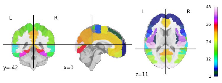
We can actually plot the atlas easily using the function plot_roi:
display = plotting.plot_roi(ho_maxprob_atlas_img, colorbar=True)
Atlas maps images#
In atlas maps images, the regions are not defined by single labels (such as in probabilistic atlases) and may overlap. An example of such as atlas map image is the original probabilistic version of the Harvard-Oxford atlas:
ho_prob_atlas = datasets.fetch_atlas_harvard_oxford('cort-prob-2mm')
pprint(ho_prob_atlas)
{'filename': '/home/runner/nilearn_data/fsl/data/atlases/HarvardOxford/HarvardOxford-cort-prob-2mm.nii.gz',
'labels': ['Background',
'Frontal Pole',
'Insular Cortex',
'Superior Frontal Gyrus',
'Middle Frontal Gyrus',
'Inferior Frontal Gyrus, pars triangularis',
'Inferior Frontal Gyrus, pars opercularis',
'Precentral Gyrus',
'Temporal Pole',
'Superior Temporal Gyrus, anterior division',
'Superior Temporal Gyrus, posterior division',
'Middle Temporal Gyrus, anterior division',
'Middle Temporal Gyrus, posterior division',
'Middle Temporal Gyrus, temporooccipital part',
'Inferior Temporal Gyrus, anterior division',
'Inferior Temporal Gyrus, posterior division',
'Inferior Temporal Gyrus, temporooccipital part',
'Postcentral Gyrus',
'Superior Parietal Lobule',
'Supramarginal Gyrus, anterior division',
'Supramarginal Gyrus, posterior division',
'Angular Gyrus',
'Lateral Occipital Cortex, superior division',
'Lateral Occipital Cortex, inferior division',
'Intracalcarine Cortex',
'Frontal Medial Cortex',
'Juxtapositional Lobule Cortex (formerly Supplementary Motor '
'Cortex)',
'Subcallosal Cortex',
'Paracingulate Gyrus',
'Cingulate Gyrus, anterior division',
'Cingulate Gyrus, posterior division',
'Precuneous Cortex',
'Cuneal Cortex',
'Frontal Orbital Cortex',
'Parahippocampal Gyrus, anterior division',
'Parahippocampal Gyrus, posterior division',
'Lingual Gyrus',
'Temporal Fusiform Cortex, anterior division',
'Temporal Fusiform Cortex, posterior division',
'Temporal Occipital Fusiform Cortex',
'Occipital Fusiform Gyrus',
'Frontal Operculum Cortex',
'Central Opercular Cortex',
'Parietal Operculum Cortex',
'Planum Polare',
"Heschl's Gyrus (includes H1 and H2)",
'Planum Temporale',
'Supracalcarine Cortex',
'Occipital Pole'],
'maps': <nibabel.nifti1.Nifti1Image object at 0x7f53f0ad76a0>}
Again, this atlas (contained in the variable ho_prob_atlas) contains both labels (ho_prob_atlas['labels']) and maps (ho_prob_atlas['maps']), like with the “maxprob” atlas, but this time, the maps image is a 4D image:
ho_prob_atlas_img = image.load_img(ho_prob_atlas['maps'])
print("ho_prob_atlas_img has shape %s" % (ho_prob_atlas_img.shape,))
ho_prob_atlas_img has shape (91, 109, 91, 48)
In this ho_prob_atlas_img, the fourth dimension now refers to the different regions! Note that there are only 48 volumes because the “background” does not get it’s own volume. Now, suppose that I would like to extract the volume corresponding to the insula (label nr. 3), we need to extract the first volume (this is because the background did get its own volume; a bit confusing, we know):
insula_prob_roi = image.index_img(ho_prob_atlas_img, 1)
print("Shape of insula ROI: %s" % (insula_prob_roi.shape,))
Shape of insula ROI: (91, 109, 91)
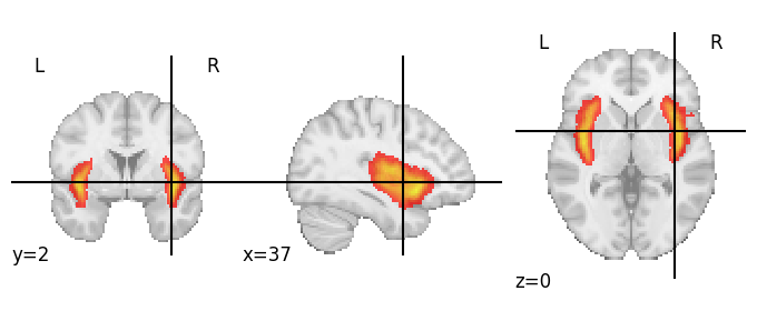
Again, we can plot this using plot_roi:
display = plotting.plot_roi(insula_prob_roi, cmap='autumn', vmin=0)
# Plot the insula ROI on the fsaverage5 surface here
# YOUR CODE HERE
raise NotImplementedError()
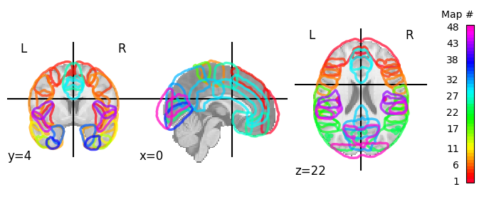
Alright, back to volume plots. Nilearn contains even a function to plot the entire probabilitic atlas (given some threshold) in a single plot: plot_probabilistic_atlas.
# This may take a couple of seconds
display = plotting.plot_prob_atlas(ho_prob_atlas_img, colorbar=True, threshold=5)
At this moment, we could use our insula ROI (after binarizing) to index our functional data (func_img), except that we have one problem: although the ROI (insula_prob_roi) and our data (func_img) are aligned, they do not have the same dimensions:
print("Affine of func_img:")
print(func_img.affine)
print("\nAffine of ROI:")
print(insula_prob_roi.affine)
Affine of func_img:
[[ 4. 0. 0. -96.]
[ 0. 4. 0. -132.]
[ 0. 0. 4. -78.]
[ 0. 0. 0. 1.]]
Affine of ROI:
[[ 2. 0. 0. -90.]
[ 0. 2. 0. -126.]
[ 0. 0. 2. -72.]
[ 0. 0. 0. 1.]]
Again, Nilearn comes to the rescue! We can use image.resample_img (or alternatively, image.resample_to_img) to resample our ROI to the resolution of our functional data. Check out the docs of the resample_img function!
(Note that we didn’t have to do this when we plotted our insula ROI on top of an MNI image background, because most plotting functions in Nilearn automatically resample the to-be-plotted data to the background image “under the hood”.)
Let’s do this below:
insula_prob_roi_resamp = image.resample_img(
insula_prob_roi,
target_affine=func_img.affine,
target_shape=func_img.shape[:3]
)
print("New affine of ROI:")
print(insula_prob_roi_resamp.affine)
New affine of ROI:
[[ 4. 0. 0. -96.]
[ 0. 4. 0. -132.]
[ 0. 0. 4. -78.]
[ 0. 0. 0. 1.]]
- Extract the probabilistic ROI of the "Temporal Pole" from the ho_prob_atlas_img variable (plot it with plot_roi to see whether you succeeded);
- Using the function image.threshold_img, threshold the probabilistic ROI at 40 (setting all voxels with the value 40 and below to zero);
- Resample the thresholded mask to the dimensions of our functional data (func_img);
- Using image.math_img, binarize the thresholded and resampled ROI (where voxels belonging to the thresholded ROI should have value 1 and 0 otherwise);
- Finally, apply this mask to the func_img variable using apply_mask (or NiftiMasker, up to you);
- Average the time series signal across the 1043 temporal pole voxel and store these values (should be an array of 176 values) in a new variable named average_tp_signal.
# Implement your ToDo here!
# YOUR CODE HERE
raise NotImplementedError()
''' Tests the above ToDo. '''
np.testing.assert_array_almost_equal(
average_tp_signal[:5],
np.array([299.29, 299.42, 299.26, 299.89, 298.79]),
decimal=2
)
print("Well done!")
If you did the previous ToDo, you noticed it took quite some lines of code to implement (but way less that you’d need when implementing it in pure Numpy!). This would take even more lines of code if you would like to do this for multiple ROIs, for example, in “connectome”-based analyses (which we’ll discuss in a bit). Fortunately, Nilearn contains several functions do this within a single line of code.
There are different functions for “atlas maps images” (such as for our probabilistic Harvard-Oxford atlas) and “atlas label images” (such as our “maxprob” Harvard-Oxford atlas). The corresponding functions that allow multi-ROI masking and averaging the signal across voxels (like you did in the previous ToDo) are img_to_signals_labels and img_to_signals_maps from the regions module, respectively. Both transform a 4D (\(X \times Y \times Z \times T\)) image to a 2D (\(T \times K\), where \(K\) is the number of regions in the atlas) numpy array.
Let’s take a look at the img_to_signals_labels function first. We’ll use our previously defined ho_maxprob_atlas_img. Importantly, we first need to resample the atlas label image to the space of our functional data (we’ll use resample_to_img this time, which is a little less “verbose” than the resample_img function):
ho_maxprob_atlas_img_resamp = image.resample_to_img(
ho_maxprob_atlas_img,
target_img=func_img,
interpolation='nearest'
)
Note that we specify that the resampling function should use “nearest neighbor” interpolation instead of the default “continuous” interpolation (otherwise labels at the edge of regions could get a value of, e.g., 3.05, while labels in atlas label images should always be whole numbers/integers).
Now, in a single line of code (`using_, we can transform our 4D image to a 2D array with the average time series (i.e., across voxels) for all ROIs in our atlas:
av_roi_data = regions.img_to_signals_labels(
func_img,
labels_img=ho_maxprob_atlas_img_resamp,
background_label=0
)
Notably, the img_to_signals_labels returns two things:
The actual average ROI signals;
The corresponding (integer) labels
av_roi_signals = av_roi_data[0]
roi_labels = av_roi_data[1]
print("average_roi_signals is a %s with shape: %s" % (type(av_roi_signals).__name__, av_roi_signals.shape))
average_roi_signals is a ndarray with shape: (168, 48)
The function for atlas maps images (img_to_signals_maps) can be used in essentially the same way as the img_to_signals_labels function, except that it should be given a atlas maps image instead.
By the way, there exists variations of the NiftiMasker class that basically does the same as the img_to_signals_{labels,maps} functions: NiftiLabelsMasker and NiftiMapsMasker. Just like the img_to_signals_labels function, this indexes our functional data with multiple ROIs in which the signal is subsequently averaged across voxels, but it also includes resampling of the atlas (if necessary) and optional preprocessing (just like the NiftiMasker class).
We’ll show you how it can be used on our data below:
from nilearn.input_data import NiftiLabelsMasker
nlm = NiftiLabelsMasker(labels_img=ho_maxprob_atlas_img)
av_roi_signals = nlm.fit_transform(func_img)
print("Shape of av_roi_signals: %s" % (av_roi_signals.shape,))
Shape of av_roi_signals: (168, 48)
Alright, now you know how to leverage the basic functionality from the regions module. Note that, in addition to the several existing anatomically and functionally defined atlases (check out the datasets module), Nilearn also contains several wrapper functions for scikit-learn functions that allow you to estimate parcellations from your own data (using, e.g., Ward clustering, Kmeans clustering, Dictionary learning or canonical ICA). But that’s something for another tutorial perhaps.
Connectome/connectivity analyses#
When we have a 2D array with average time series of multiple ROIs, we can easily implement a “connectome”-based analysis using the connectome module of Nilearn. This module has several functions/classes that allow you to estimate “functional connectomes”, which are basically connectivity matrices based on a similarity measure (such as correlation) between time series across ROIs. As such, these matrices have a \(K \times K\) shape (where \(K\) reflects the number of ROIs). From these connectivity matrices, in turn, you could for example perform network analyses.
There are different classes for connectome estimation, including ConnectivityMeasure (a general-purpose connectivity estimator), GroupSparseCovariance and GroupSparseCovarianceCV (estimators for specific “sparse” connectivity matrices across multiple subjects).
For now, we’ll focus on the general ConnectivityMeasure class. We’ll start by importing it:
from nilearn.connectome import ConnectivityMeasure
As you can see in the docs, the ConnectivityMeasure class has the “initialize-fit-transform” structure. For our purposes here, the most important argument upon initialization of the class is the kind argument, which specifies the particular connectivity measure (“correlation”, “partial correlation”, “tangent”, “covariance”, or “precision”). We will use the default values for the other arguments.
cm = ConnectivityMeasure(kind='correlation')
Now, just as the NiftiMasker class, you need to call both the fit and tranform methods (or the fit_transform method for convenience) to actually estimate and return the \(K \times K\) connectivity matrix (or matrices, if you have multiple subjects). Importantly, the fit and transform (and fit_transform) methods take a list of numpy arrays (of shape \(T \times K\), where \(T\) represents the number of time points and \(K\) the number of ROIs) representing the individual subjects’ data. These functions output a \(N \times K \times K\) array, representing a \(K \times K\) connectivity matrix for all \(N\) subjects.
Here, we only have data from a single subject (contained in the av_roi_signals variable), so we’ll supply the fit_transform function with a list containing a single array. As such, the output will be a \(1 \times K \times K\) array:
corr_mat = cm.fit_transform([av_roi_signals]) # input = list with single matrix
print("corr_mat is a 2D array with shape: %s" % (corr_mat.shape,))
corr_mat is a 2D array with shape: (1, 48, 48)
As we only a have single subject, let’s “squeeze” out the singleton dimension:
corr_mat = corr_mat.squeeze()
print("corr_mat now has the following shape: %s" % (corr_mat.shape,))
corr_mat now has the following shape: (48, 48)
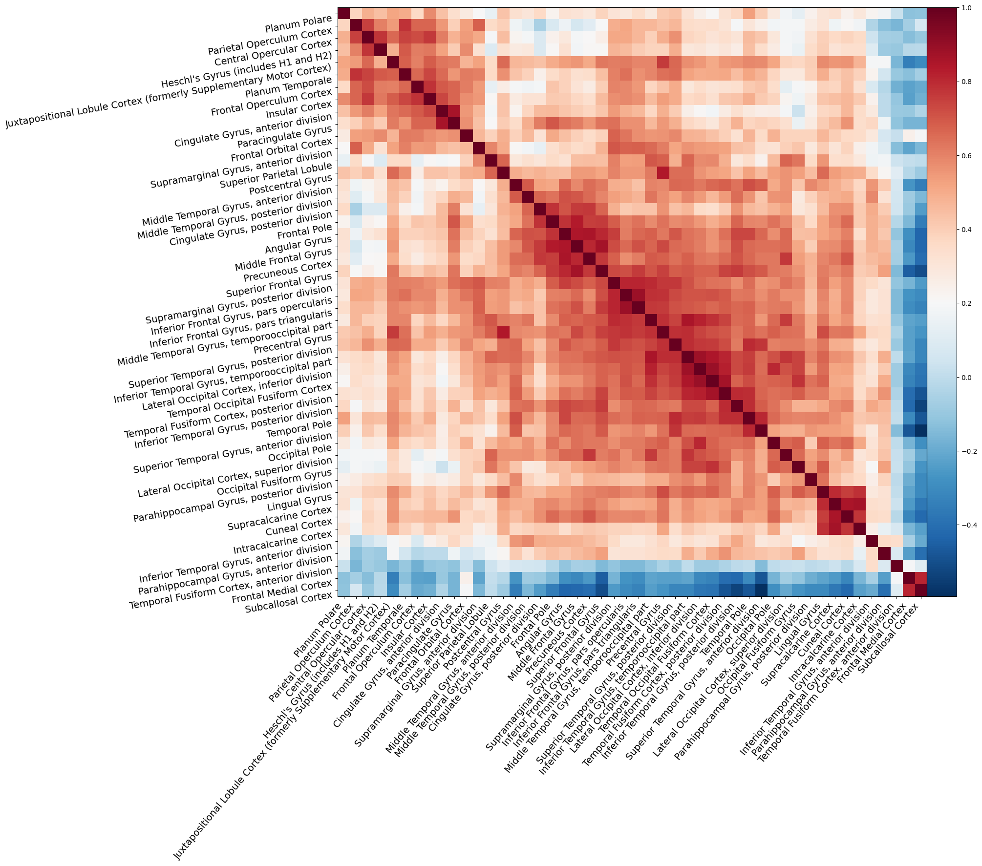
Now, on the matrix (corr_mat) you could, for example, perform additional network-analyses or just visualize it, either the matrix itself or as a network of brain regions on top of a brain.
First, we’ll show how to plot the matrix. We’ll use the plotting.plot_matrix function for this. Because the labels are barely readable with the default plot size, we’ll create a Matplotlib figure beforehand and pass it to the plotting function:
import matplotlib.pyplot as plt
fig, ax = plt.subplots(figsize=(15, 15))
display = plotting.plot_matrix(
corr_mat,
labels=ho_maxprob_atlas['labels'][1:],
reorder='average',
figure=fig
)
# Increase the labels a bit
display.axes.tick_params(axis='both', which='major', labelsize=14)
We can also create a visualization of the network of brain regions on top of a (transparent) background (MNI) brain using plotting.plot_connectome, or even an interactive version using plotting.view_connectome. Importantly, these functions need to know the (peak) MNI coordinates of the regions from the atlas that you used. Sometimes, these are included in the atlas (as a separate entry into the data dictionary, next to “maps” and “labels”), but if not, you can extract them using the plotting.find_parcellation_cut_coords function:
coords = plotting.find_parcellation_cut_coords(ho_maxprob_atlas_img)
Now, let’s create an interactive connectome plot. We’ll set the edge_threshold to 90%, which will show only the edges with the 10% highest connectivity values (otherwise, the plot will become a bit cluttered):
plotting.view_connectome(
corr_mat,
coords,
edge_threshold="90%"
)
Note that the view_connectome function only plots the graph edges (i.e., the correlation values) on the left hemisphere (although the nodes represent bilateral ROIs).
Try the following:
- Using the NiftiLabelsMasker class, perform sensible preprocessing (e.g., high-pass filtering and smoothing) and regress out the confounds (in data['confounds'] by passing it to the fit function;
- Estimate the connectivity matrix again;
- Visualize the connectivity matrix and interactive connectome plot again
Note that few people seem to agree on the best ways to preprocess fMRI data for network analyses. If you ever want to do these type of analyses, we recommend checking the literature!
# Implement the ToDo here
# YOUR CODE HERE
raise NotImplementedError()
Concluding remarks#
We covered quite some functionality from the Nilearn package, but definitely not all! It als contains some useful features for “decoding” analyses (in the decoding module, including a class to perform Searchlight-based analysis and several classifiers for spatially-structured data such as fMRI data) amongst other things.
We highly recommend you browse through the ample excellent tutorials and examples on the Nilearn website, which cover other and more advanced usecases than discussed in this tutorial.
That said, we hope that this tutorial helps you to get started with your analyses using Nilearn.
Happy hacking!