
The GLM, part 2: inference#
In this notebook, we’ll continue with the GLM, focusing on statistical tests (i.e., inference) of parameters. Note that there are two notebooks this week: this one, glm_part2_inference.ipynb, and design_of_experiments.ipynb. Please do this one first.
Last week, you learned how to estimate parameters of the GLM and how to interpret them. This week, we’ll focus on statistical inference of those estimated parameters (and design of experiment, in another notebook). Importantly, we are going to introduce the most important formula in the context of univariate fMRI analyses: the formula for the t-value. Make sure you understand this formula, as we will continue to discuss it in the next weeks.
What you’ll learn: after this week’s lab …
you know how the different parts of the t-value formula and how they relate to your data and experiment;
you are able to calculate t-values and corresponding p-value of parameters from a GLM;
Estimated time needed to complete: 1-3 hours
# First some imports
import numpy as np
import matplotlib.pyplot as plt
from numpy.linalg import inv
%matplotlib inline
Introduction#
From your statistics classes, you might remember that many software packages (e.g. SPSS, R, SAS) do not only return beta-parameters of linear regression models, but also t-values and p-values associated with those parameters. These statistics evaluate whether a beta-parameter (or combination of beta-parameters) differs significantly from 0 (or in fMRI terms: whether a voxel activates/deactivates significantly in response to one or more experimental factors).
In univariate (activation-based) fMRI studies, we need statistics to evaluate the estimated parameters in context of the uncertainty of their estimation. As we’ll discuss later in more detail, interpreting (and performing inference about) the magnitude of GLM parameters without their associated uncertainty is rarely warranted in univariate fMRI studies. To illustrate the problem with this, let’s look at an example.
In this example, we try to predict someone’s height (in meters; \(\mathbf{y}\)) using someone’s weight (in kilos; \(\mathbf{X}\)). (Note that the data is not necessarily representative of the true relationship between height and weight.)
Anyway, let’s run a linear regression using weight (in kilos) as a predictor for height (in meters).
data = np.load('weight_height_data.npz')
X, y = data['X'], data['y']

plt.figure(figsize=(10, 6))
plt.scatter(X, y)
plt.title('Relation between weight and height (in meters)', y=1.05, fontsize=20)
plt.xlabel('Weight (kg)', fontsize=20)
plt.ylabel('Height (meters)', fontsize=20)

Xn = np.hstack((np.ones((y.size, 1)), X))
beta = inv(Xn.T @ Xn) @ Xn.T @ y
y_hat = Xn @ beta
mse = np.mean((y_hat - y) ** 2)
plt.plot([X.min(), X.max()], [Xn.min(axis=0) @ beta, Xn.max(axis=0) @ beta], ls='-', c='r')
plt.xlim((X.min(), X.max()))
plt.text(70, 1.9, r'$\hat{\beta}_{weight} = %.5f$' % beta[1], fontsize=18)
plt.text(70, 1.8, r'$MSE = %.5f$' % mse, fontsize=18)
plt.grid()

plt.show()
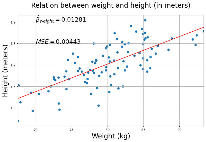
Well, quite a modest beta-parameter on the one hand, but on the other hand the Mean Squared Error is also quite low. Now, to illustrate the problem of interpretating ‘raw’ beta-weights, let’s rephrase our objective of predicting height based on weight: we’ll try to predict height in centimeters based on weight (still in kilos). So, what we’ll do is just rescale the data points of \(\mathbf{y}\) (height in meters) so that they reflect height in centimeters. We can simply do this by multipling our \(\mathbf{y}\) by 100.
y_cm = y * 100
Now, you wouldn’t expect our model to change, right? We only rescaled our target … As you’ll see below, this actually changes a lot!
''' Implement the ToDo here. '''

# YOUR CODE HERE
raise NotImplementedError()
print(beta_cm)
''' Tests the above ToDo'''
np.testing.assert_almost_equal(beta_cm, beta * 100, decimal=4)
np.testing.assert_almost_equal(mse_cm, mse * 10000, decimal=4)
print("Well done!")
If you did it correctly, when you compare the beta-parameters between the two models (one where \(y\) is in meters, and one where \(y\) is in centimeters), you see a massive difference — a 100 fold difference to be exact*! This is a nice example where you see that the (raw) value of the beta-parameter is completely dependent on the scale of your variables. (Actually, you could either rescale \(\mathbf{X}\) or \(\mathbf{y}\)); both will have a similar effect on your estimated beta-parameter.)
Think of (at least) two reasons why voxels might differ in their scale and write them down in the text cell below.
YOUR ANSWER HERE
How to compute t-values and p-values#
So, you’ve seen that interpreting beta-parameters by themselves is useless because their value depends very much on the scale of your variables. But how should we, then, interpret the effects of our predictors on our target-variable? From the plots above, you probably guessed already that it has something to do with the MSE of our model (or, more generally, the model fit). That is indeed the case. As you might have noticed, not only the beta-parameters depend on the scale of your data, the errors (residuals) depend on the scale as well. In other words, not only the effect (beta-values) but also the noise (errors, MSE) depend on the scale of the variables!
t-values#
In fact, the key to getting interpretable effects of our predictors is to divide (“normalize”) our beta-parameter(s) by some quantity that summarizes how well our model describes the data. This quantity is the standard error of the beta-parameter, usually denoted by \(\mathrm{SE}_{\beta}\). The standard error of the beta-parameter can be computed by taking the square root of the variance of the beta-parameter. If we’d divide our beta-estimate with it’s standard error, we compute a statistic you are all familiar with: the t-statistic! Formally:
Another way to think about it is that the t-value is the “effect” (\(\hat{\beta}\)) divided by your (un)certainty or confidence in the effect (\(\mathrm{SE}_{\hat{\beta}}\)). In a way, you can think of t-values as “uncertainty-normalized” effects.
So, what drives (statistical) uncertainty about “effects” (here: \(\hat{\beta}\) parameters)? To find out, let’s dissect the uncertainty term, \(\mathrm{SE}_{\hat{\beta}}\), a little more. The standard error of a parameter can interpreted conceptually as the “unexplained variance of the model” (or noise) multiplied with the “design variance” (or: the variance of the parameter due to the design). In this lab, we won’t explain what design variance means or how to compute this, as this is the topic of the second notebook of this week (design_of_experiments).
For now, we treat “design variance”, here, as some known (constant) value given the design matrix (\(\mathbf{X}\)). So, with this information, we can construct a conceptual formula for the standard error of our parameter(s):
Now we also create a “conceptual formula” for the t-statistic:
This (conceptual) formula involving effects, noise, and design variance is probably the most important concept of this course. The effects (t-values) we measure in GLM analyses of fMRI data depend on two things: the effect measured (\(\hat{\beta}\)) and the (un)certainty of the effect (\(SE_{\hat{\beta}}\)), of which the latter term can be divided into the unexplained variance (“noise”) and the design variance (uncertainty of the parameter due to the design).
These two terms (noise and design variance) will be central to the next couple of weeks of this course. In this week’s second notebook (topic: design of experiments), we’ll focus on how to optimize our t-values by minimizing the “design variance” term. Next week (topic: preprocessing), we’ll focus on how to (further) optimize our t-values by minimizing the error/noise.
While we’re going to ignore the design variance for now, we are, however, going to learn how to calculate the “noise” term.
In fact, the noise term is very similar to the MSE, but instead of taking the mean of the squared residuals, we sum the squared residuals (“sums of squared erros”, SSE) and divide it by the model’s degrees of freedom (DF). People usually use the \(\hat{\sigma}^{2}\) symbol for this noise term:
where the degrees of freedom (df) are defined as the number of samples (\(N\)) minus the number of predictors including the intercept (\(P\)):
So, the formula of the t-statistic becomes:
Alright, enough formulas. Let’s see how we can compute these terms in Python. We’re going to calculate the t-statistic of the weight-predictor for both models (the meter and the centimeter model) to see whether we can show that essentially the (normalized) effect of weight on height in meters is the same as the effect on height in centimeters; in other words, we are going to investigate whether the conversion to t-values “normalizes” the beta-parameters.
First, we’ll create a function for you to calculate the design-variance. You don’t have to understand how this works; we’re going to explain this to you in detail next week.
def design_variance(X, which_predictor=1):
    ''' Returns the design variance of a predictor (or contrast) in X.

    Parameters
    ----------
    X : numpy array
        Array of shape (N, P)
    which_predictor : int or list/array
        The index of the predictor you want the design var from.
        Note that 0 refers to the intercept!
        Alternatively, "which_predictor" can be a contrast-vector
        (which will be discussed later this lab).

    Returns
    -------
    des_var : float
        Design variance of the specified predictor/contrast from X.
    '''

    is_single = isinstance(which_predictor, int)
    if is_single:
        idx = which_predictor
    else:
        idx = np.array(which_predictor) != 0

    c = np.zeros(X.shape[1])
    c[idx] = 1 if is_single == 1 else which_predictor[idx]
    des_var = c.dot(np.linalg.inv(X.T.dot(X))).dot(c.T)
    return des_var
So, if you want the design variance of the ‘weight’ parameter in the varianble Xn from before, you do:
# use which_predictor=1, because the weight-column in Xn is at index 1 (index 0 = intercept)
design_variance_weight_predictor = design_variance(Xn, which_predictor=1)
print("Design variance of weight predictor is: %.6f " % design_variance_weight_predictor)
Design variance of weight predictor is: 0.000334
Alright, now we only need to calculate our noise-term (\(\hat{\sigma}^2\)):
# Let's just redo the linear regression (for clarity)
beta_meter = inv(Xn.T @ Xn) @ Xn.T @ y
y_hat_meter = Xn @ beta_meter

N = y.size
P = Xn.shape[1]
df = (N - P)
print("Degrees of freedom: %i" % df)
sigma_hat = np.sum((y - y_hat_meter) ** 2) / df
print("Sigma-hat (noise) is: %.3f" % sigma_hat)
design_variance_weight = design_variance(Xn, 1)
Degrees of freedom: 98
Sigma-hat (noise) is: 0.005
Now we can calculate the t-value:
t_meter = beta_meter[1] / np.sqrt(sigma_hat * design_variance_weight)
print("The t-value for the weight-parameter (beta = %.3f) is: %.3f" % (beta_meter[1], t_meter))
The t-value for the weight-parameter (beta = 0.013) is: 10.431
That’s it! There’s not much more to calculating t-values in linear regression. Now it’s up to you to do the same thing and calculate the t-value for the model of height in centimeters, and check if it is the same as the t-value for the weight parameter in the model with height in meters.
''' Implement your ToDo here. '''

# YOUR CODE HERE
raise NotImplementedError()
''' Tests the above ToDo. '''
try:
    np.testing.assert_almost_equal(t_centimeter, t_meter)
except AssertionError as e:
    print("The t-value using height in centimeters is not the same as when using height in meters!")
    raise(e)

print("Well done!")
P-values#
As you can see, calculating t-values solves the “problem” of uninterpretable beta-parameters!
Now, the last thing you need to know is how to calculate the statistical significance of your t-value, or in other words, how you calculate the corresponding p-value. You probably remember that the p-value corresponds to the area under the curve of a t-distribution associated with your observed t-value and more extreme values:
 Image credits: Frank Dietrich and Mike Collins, Northern Kentucky University
The function stats.t.sf(t_value, df) from the scipy package does exactly this. Importantly, this function always returns the right-tailed p-value. For negative t-values, however, you’d want the left-tailed p-value. One way to remedy this, is to always pass the absolute value of your t-value - np.abs(t_value) to the stats.t.sf() function. Also, the stats.t.sf() function by default returns the one-sided p-value. If you’d want the two-sided p-value, you can simply multiply the returned p-value by two to get the corresponding two-sided p-value.
Let’s see how we’d do that in practice:
from scipy import stats

# take the absolute by np.abs(t)
p_value = stats.t.sf(np.abs(t_meter), df) * 2 # multiply by two to create a two-tailed p-value
print('The p-value corresponding to t(%i) = %.3f is: %.8f' % (df, t_meter, p_value))
The p-value corresponding to t(98) = 10.431 is: 0.00000000
Contrasts#
We’re almost done! We’re really at 99% of what you should know about the GLM and fMRI analysis (except for some important caveats that have to do with GLM assumptions, that we’ll discuss next week). The only major concept that we need to discuss is contrasts. Contrasts are basically follow-up statistical tests of GLM parameters, with which you can implement any (linear) statistical test that you are familiar with. t-tests, F-tests, ANCOVAs — they can all be realized with the GLM and the right contrast(s). (Again, if you want to know more about this equivalence between the GLM and common statistical tests, check out this blog post.) Importantly, the choice of contrast should reflect the hypothesis that you want to test.
t-tests#
T-tests in the GLM can be implemented in two general ways:
1. Using a contrast of a parameters “against baseline”
This type of contrast basically tests the hypothesis: “Does my predictor have any effect on my dependent variable?” In other words, it tests the following hypothesis:
\(H_{0}: \beta = 0\) (our null-hypothesis, i.e. no effect)
\(H_{a}: \beta \neq 0\) (our two-sided alternative hypothesis, i.e. some effect)
Note that a directional alternative hypothesis is also possible, i.e., \(H_{a}: \beta > 0\) or \(H_{a}: \beta < 0\).
2. Using a contrast between parameters
This type of contrast basically tests hypotheses such as “Does predictor 1 have a larger effect on my dependent variable than predictor 2?”. In other words, it tests the following hypothesis:
\(H_{0}: \beta_{1} - \beta_{2} = 0\) (our null-hypothesis, i.e. there is no difference)
\(H_{a}: \beta_{1} - \beta_{2} \neq 0\) (our alternative hypothesis, i.e. there is some difference)
Let’s look at an example of how we would evaluate a simple hypothesis that a beta has an some effect on the dependent variable. Say we’d have an experimental design with 6 conditions:
condition 1: images of male faces with a happy expression
condition 2: images of male faces with a sad expression
condition 3: images of male faces with a neutral expression
condition 4: images of female faces with a happy expression
condition 5: images of female faces with a sad expression
condition 6: images of female faces with a neutral expression
Let’s assume we have fMRI data from a run with 100 volumes. We then have a target-signal of shape (\(100,\)) and a design-matrix (after convolution with a canonical HRF) of shape (\(100 \times 7\)) (the first predictor is the intercept!). We load in this data below:
data = np.load('data_contrast_example.npz')
X, y = data['X'], data['y']

print("Shape of X: %s" % (X.shape,))
print("Shape of y: %s" % (y.shape,))
Shape of X: (100, 7)
Shape of y: (100,)
After performing linear regression with these 6 predictors (after convolving the stimulus-onset times with an HRF, etc. etc.), you end up with 7 beta values:
betas = inv(X.T @ X) @ X.T @ y
betas = betas.squeeze()  # remove singleton dimension; this is important for later
print("Betas corresonding to our 6 conditions (and intercept):\n%r" % betas.T)
Betas corresonding to our 6 conditions (and intercept):
array([ 0.08208567, -0.21982422, -0.16284892,  0.53208935,  0.26214462,
        0.38945094,  0.21565532])
The first beta corresponds to the intercept, the second beta to the male/happy predictor, the third beta to the male/sad predictor, etc. etc. Now, suppose that we’d like to test whether images of male faces with a sad expression have an influence on voxel activity (our dependent variable).
The first thing you need to do is extract this particular beta value from the array with beta values (I know this sounds really trivial, but bear with me):
beta_male_sad = betas[2]
print("The 'extracted' beta is %.3f" % beta_male_sad)
The 'extracted' beta is -0.163
In neuroimaging analyses, however, this is usually done slightly differently: using contrast-vectors. Basically, it specifies your specific hypothesis about your beta(s) of interest in a vector. Before explaining it in more detail, let’s look at it in a code example:
# Again, we'd want to test whether the beta of "male_sad" is different from 0
contrast_vector = np.array([0, 0, 1, 0, 0, 0, 0])
contrast = (betas * contrast_vector).sum() # we simply elementwise multiply the contrast-vector with the betas and sum it!
print('The beta-contrast is: %.3f' % contrast)
The beta-contrast is: -0.163
“Wow, what a tedious way to just select the third value of the beta-array”, you might think. And, in a way, this is indeed somewhat tedious for a contrast against baseline. But let’s look at a case where you would want to investigate whether two betas are different - let’s say whether male sad faces have a larger effect on our voxel than male happy faces. Again, you could do this:
beta_difference = betas[2] - betas[1]
print("Difference between betas: %.3f" % beta_difference)
Difference between betas: 0.057
… but you could also use a contrast-vector:
contrast_vector = np.array([0, -1, 1, 0, 0, 0, 0])
contrast = (betas * contrast_vector).sum()
print('The contrast between beta 2 and beta 1 is: %.3f' % contrast)
print('This is exactly the same as beta[2] - beta[1]: %.3f' % (betas[2]-betas[1]))
The contrast between beta 2 and beta 1 is: 0.057
This is exactly the same as beta[2] - beta[1]: 0.057
“Alright, so using contrast-vectors is just a fancy way of extracting and subtracting betas from each other …”, you might think. In a way, that’s true. But you have to realize that once the hypotheses you want to test become more complicated, using contrast-vectors actually starts to make sense.
Let’s look at some more elaborate hypotheses. First, let’s test whether male faces lead to higher voxel activity than female faces, regardless of emotion:
# male faces > female faces
contrast_vector = [0, 1, 1, 1, -1, -1, -1]
male_female_contrast = (contrast_vector * betas).sum()
print("Male - female contrast (regardless of expression): %.2f" % male_female_contrast)
Male - female contrast (regardless of expression): -0.72
… or whether emotional faces (regardless of which exact emotion) lead to higher activity than neutral faces:
# Emotion (regardless of which emotion, i.e., regardless of sad/happy) - neutral
contrast_vector = np.array([0, 1, 1, -2, 1, 1, -2])
emo_neutral_contrast = (contrast_vector * betas).sum()
print("Emotion - neutral contrast (regardless of which emotion): %.2f" % emo_neutral_contrast)
Emotion - neutral contrast (regardless of which emotion): -1.23
See how contrast-vectors come in handy when calculating (more intricate) comparisons? In the male-female contrast, for example, instead ‘manually’ picking out the betas of ‘sad_male’ and ‘happy_male’, averaging them, and subtracting their average beta from the average ‘female’ betas (‘happy_female’, ‘sad_female’), you can specify a contrast-vector, multiply it with your betas, and sum them. That’s it.
YOUR ANSWER HERE
# Implement the sad - neutral contrast here:

# YOUR CODE HERE
raise NotImplementedError()
''' Tests the above ToDo. '''
from niedu.tests.nii.week_3 import test_contrast_todo_1
test_contrast_todo_1(betas, contrast_todo)
We’re not only telling you about contrasts because we think it’s an elegant way of computing beta-comparisons, but also because virtually every major neuroimaging software package uses them, so that you can specify what hypotheses you exactly want to test! You’ll also see this when we’re going to work with FSL (in week 5) to perform automated whole-brain linear regression analyses.
Knowing how contrast-vectors work, we now can extend our formula for t-tests of beta-parameters such that they can describe every possible test (not only t-tests, but also ANOVAs, F-tests, etc.) of betas “against baseline” or between betas that you can think of:
Our “old” formula of the t-test of a beta-parameter:
And now our “generalized” version of the t-test of any contrast/hypothesis:
in which \(\mathbf{c}\) represents the entire contrast-vector, and \(c_{j}\) represents the \(j^{\mathrm{th}}\) value in our contrast vector. By the way, we can simplify the (notation of the) numerator a little bit using some matrix algebra. Remember that multiplying two (equal length) vectors with each other and then summing the values together is the same thing as the (inner) “dot product” between the two vectors?
This means that you can also evaluate this elementwise multiplication and sum of the contrast-vector and the betas using the dot-product:
some_betas = np.array([1.23, 2.95, 3.33, 4.19])
some_cvec = np.array([1, 1, -1, -1])

# Try to implement both approaches and convince yourself that it's
# mathematically the same!
So, you need the contrast vector in the numerator of the t-value formula (i.e., \(\mathbf{c}\hat{\beta}\)), but it turns out that you actually also need the contrast-vector in the denominator, because it’s part of the calculation of design variance. Again, we will discuss how this works exactly in the next notebook. In the function design_variance, it is also possible to calculate design variance for a particular contrast (not just a single predictor) by passing a contrast vector to the which_predictor argument.
We’ll show this below:
# E.g., get design-variance of happy/male - sad/male
c_vec = np.array([0, 1, -1, 0, 0, 0, 0])  # our contrast vector!
dvar = design_variance(X, which_predictor=c_vec)  # pass c_vec to which_predictor
print("Design variance of happy/male - sad/male: %.3f" % dvar)
Design variance of happy/male - sad/male: 0.024
For the rest of ToDos this lab, make sure to pass your contrast-vector to the design_variance function in order to calculate it correctly.
Now you know enough to do it yourself!
Calculate the t-value and p-value for the hypothesis “sad faces have a larger effect than happy faces (regardless of gender) on our dependent variable” (i.e. voxel activity). In other words, test the hypothesis: \(\beta_{sad} - \beta_{happy} \neq 0\) (note that this is a two-sided test!).
Store the t-value and p-value in the variables tval_todo and pval_todo respectively. We reload the variables below (we’ll call them X_new and y_new) to make sure you’re working with the correct data. Note that the X_new variable already contains an intercept; the other six columns correspond to the different predictors (male/hapy, male/sad, etc.). In summary, you have to do the following:
(you don’t have to calculate the betas; this has already been done (stored in the variable betas)
calculate “sigma-hat” (\(\mathrm{SSE} / \mathrm{df}\))
calculate design-variance (use the design_variance function with a proper contrast-vector)
calculate the contrast (\(\mathbf{c}\hat{\beta}\))
calculate the t-value and p-value
data = np.load('data_contrast_example.npz')
X_new, y_new = data['X'], data['y']

print("Shape of X: %s" % (X_new.shape,))
print("Shape of y: %s" % (y_new.shape,))

# YOUR CODE HERE
raise NotImplementedError()
''' Part 1 of testing the above ToDo. '''
from niedu.tests.nii.week_3 import test_contrast_todo_2
test_contrast_todo_2(X_new, y_new, betas, tval_todo, pval_todo)
print("Well done!")
F-tests on contrasts#
In the previous section we discussed how to calculate t-values for single contrasts. However, sometimes you might have a hypothesis about multiple contrasts at the same time. This may sound weird, but let’s consider an experiment.
Suppose you have data from an experiment in which you showed images of circles which were either blue, red, or green. In that case, you have three predictors. Then, you could have very specific question, like “Do blue circles activate a voxel significantly compared to baseline”, which corresponds to the following null and alternative hypothesis:
\(H_{0}: \beta_{blue} = 0\) (our null-hypothesis, i.e. there is no activation compared to baseline)
\(H_{a}: \beta_{blue} > 0\) (our alternative hypothesis, i.e. blue activates relative to baseline)
However, you can also have a more general question, like “Does the presentation of any circle (regardless of color) activate a voxel compared to baseline?”. This question represents the following null and alternative hypothesis:
\(H_{0}: \beta_{blue} = \beta_{red} = \beta_{green} = 0\)
\(H_{a}: (\beta_{blue} > 0) \vee (\beta_{red} > 0) \vee (\beta_{green} > 0)\)
The \(\vee\) symbol in the alternative hypothesis means “or”. So the alternative hypothesis nicely illustrates our question: is there any condition (circle) that activates a voxel more than baseline? This hypothesis-test might sound familiar, because it encompasses the F-test! In other words, an F-test tests a collection of contrasts together. In the example here, the F-test tests the following contrasts together (ignoring the intercept) of our beta-parameters:
[1, 0, 0](\(\mathrm{red} > 0\))[0, 1, 0](\(\mathrm{blue} > 0\))[0, 0, 1](\(\mathrm{green} > 0\))
Thus, a F-test basically tests this contrast-matrix all at once! Therefore, the F-tests is a type of “omnibus test”!
Now, let’s look at the math behind the F-statistic. The F-statistic for set of \(K\) contrasts (i.e., the number of rows in the contrast-matrix) is defined as follows:
With a little imagination, you can see how the F-test is an extension of the t-test of a single contrast to accomodate testing a set of contrasts together. Don’t worry, you don’t have to understand how the formula for the F-statistic works mathematically and you don’t have to implement this in Python. But you do need to understand what type of hypothesis an F-test tests!
Let’s practice this in a ToDo!
Remember the temporal basis sets from before? Suppose we have an experiment with two conditions (“A” and “B”) and suppose we’ve created a design matrix based on convolution with a single-gamma basis set (with a canonical HRF, its temporal derivative, and its dispersion derivative). Together with the intercept, the design matrix thus has 7 columns (2 conditions * 3 HRF + intercept).
The order of the columns is as follows:
column 1: intercept
column 2: canonical HRF “A”
column 3: temporal deriv “A”
column 4: dispersion deriv “A”
column 5: canonical HRF “B”
column 6: temporal deriv “B”
column 7: dispersion deriv “B”
Suppose I want to test whether there is any difference in response to condition “A” (\(A > 0\)) compared to baseline, and I don’t care what element of the HRF caused it. I can use an F-test for this. What would the corresponding contrast-matrix (in which each row represents a different contrast) look like?
We’ve created an ‘empty’ (all-zeros) 2D matrix below with three rows. It’s up to you to fill in the matrix such that it can be used to test the above question/hypothesis.
# Fill in the correct values!
contrast_matrix = np.array([

    [0, 0, 0, 0, 0, 0, 0],
    [0, 0, 0, 0, 0, 0, 0],
    [0, 0, 0, 0, 0, 0, 0]

])

# YOUR CODE HERE
raise NotImplementedError()
''' Tests the above ToDo. '''
from niedu.tests.nii.week_3 import test_definition_ftest

test_definition_ftest(contrast_matrix)
print("Well done!")
Summary#
Alright, now you know basically everything about how to perform a univariate fMRI analysis!
“Wait, that’s it?”, you might ask (or not). Well, yeah, regular univariate analyses as you might read about in scientific journals do basically what you’ve just learned, but then not on a single voxel, but on each voxel in the brain separately. Basically just a gigantic for-loop across voxels in which everytime the same design (\(\mathbf{X}\)) is used to predict a new voxel-signal (\(\mathbf{y}\)). Afterwards, the t-values of the contrast (hypothesis) you’re interested in are plotted back onto a brain, color-code it (high t-values yellow, low t-values red), and voilà, you have your pretty brain plot.
YOUR ANSWER HERE
# Implement the assignment here

# YOUR CODE HERE
raise NotImplementedError()
''' Tests the above ToDo. '''
from niedu.tests.nii.week_3 import test_rest_vs_stim_contrast
test_rest_vs_stim_contrast(cvec_rest)