7 Affective face perception integrates both static and dynamic information

---

Abstract

Facial movements are crucial for affective face perception, yet research has shown that people are also influenced by features of the static face such as facial morphology. Most studies have either manipulated dynamic features (i.e., facial movements) or static features (i.e., facial morphology) making it impossible to evaluate the relative contribution of either. The current study investigates the effects of static and dynamic facial features on three affective properties (categorical emotion, valence, and arousal) inferred from stimuli in which both types of features have been independently manipulated. Using predictive machine learning models, we show that static and dynamic features both explain substantial and orthogonal variance in categorical emotion and valence ratings, while arousal ratings are only predicted accurately using dynamic, but not static, features. Moreover, using a multivariate reverse correlation approach, we show that static and dynamic features communicating the same affective property (e.g., categorical emotions) are manifested differently in the face. Our results demonstrate that in order to understand affective face perception, both facial morphology and facial movements should be considered independently.

7.1 Introduction

Faces are an important element of our daily life; faces communicate affective states of others and elicit feelings in ourselves. We might infer that someone is happy when she raises the corners of her mouth and wrinkles her eyes and we might feel unpleasant when confronted with a disapproving frown. Faces convey such impressions through facial movements, which are thought to be the primary instrument to express and communicate affective states to others (Jack & Schyns, 2015). Nevertheless, most research on affective face perception has used static depictions of facial expressions in which only the peak of the expression is shown. As such, facial movements in static stimuli are not directly observed but have to be inferred. Furthermore, although facial movements are arguably the primary drivers of how we perceive and are affected by others’ faces, studies have argued that facial movements alone are unlikely to capture all variation in how we perceive and are affected by others’ faces (Barrett et al., 2019; Snoek et al., n.d.). One possible additional source of information that may complement the dynamic information conveyed by facial movements is the static, or “neutral”, face. Although the static face is unrelated to the expressor’s affective state, studies have shown that features of the static face, such as facial morphology and complexion, in fact influence how we perceive and experience faces (Hess, Adams, & Kleck, 2009; Neth & Martinez, 2009). Although much research has examined both static features and dynamic features in the context of affective face perception (reviewed below), they have never been manipulated and compared using the same stimuli in the same experiment. In the current study, we seek to investigate, quantify, and disentangle the relative contribution of these static and dynamic facial features to affective face perception.

The attempts to relate specific facial movements to affective states go back as far as Charles Darwin’s descriptions of stereotypical facial expressions associated with categorical emotions (Darwin, 1872). Since Darwin, more quantitative efforts have been made to establish robust associations between facial movements and affective states, and categorical emotions in particular. An important development that facilitated these efforts was the Facial Action Coding System (FACS; Ekman & Friesen, 1976), which outlines a way to systematically measure, quantify, and categorize facial movements into components called “action units” (AUs). Using FACS, studies have investigated and proposed specific configurations of facial movements associated with affective states such as categorical emotions (Jack et al., 2014, 2012; Wegrzyn et al., 2017), valence and arousal (Höfling et al., 2020; Liu et al., 2020), and pain (Chen et al., 2018; Kunz et al., 2019; for a comprehensive overview, see Barrett et al., 2019). Moreover, advances in computer vision spurred the development of algorithms that are able to classify affective states based on action units (J. Cohn & Kanade, 2007; Lien et al., 1998) or other facial features such as facial landmarks (Toisoul et al., 2021) or geometric features (Barman & Dutta, 2019; Murugappan & Mutawa, 2021).

Despite the fact that facial features arguably need to be dynamic to communicate affective states, static morphological features of the face have been found to influence, or “bias”, how people interpret others’ faces. This claim is supported by research showing that people can perceive emotions in neutral (i.e., non-expressive) faces that by definition only contain static but no dynamic features. Such an effect has been demonstrated by manipulating structural features of neutral faces, where, for example, a neutral face with a lower nose and mouth or higher eyebrows was more likely to be perceived as sad (Neth & Martinez, 2009; see also Franklin et al., 2019). Similar effects have been observed in relation to certain demographics (gender, ethnicity, or age) or social judgements (e.g., dominance) that are associated with specific variations in facial morphology. For instance, research has shown that neutral male faces are more likely to be perceived as angry than neutral female faces (Adams et al., 2016; Brooks et al., 2018; Craig & Lipp, 2018) and people perceive fewer and less intense emotions in older faces relative to younger faces (reviewed in Fölster et al., 2014). The dominant explanation for these affective inferences from static faces is that these effects are driven by the visual resemblance of static features (e.g., a relatively low brow) to dynamic features associated with a particular affective state (e.g., lowering one’s brow as part of an anger expression; Hess, Adams, & Kleck, 2009; Said et al., 2009; Zebrowitz, 2017; but see Gill et al., 2014; Guan et al., 2018).

As discussed, many studies have investigated dynamic and static features that underlie affective face perception. However, because these studies usually manipulate either dynamic facial movements (Jack et al., 2014, 2009) or static facial features (Franklin et al., 2019; Neth & Martinez, 2009; for an exception, see Gill et al., 2014), the relative contribution of dynamic and static information remains unknown. In addition, studies investigating the effect of dynamic features (such as AUs) on affective face processing often use static stimuli (i.e., images; Krumhuber et al., 2013) which only shows the “peak” of the expression. The use of such static stimuli means facial movements are not directly visible and need to be inferred. As a consequence, in such studies the effect of dynamic and static features on affective face perception are fundamentally confounded. For example, a participant cannot know if a relatively low eyebrow is low because of a facial muscle movement or just because of the structure of the face. This potential confound of static features is even more problematic in automated facial emotion recognition systems, which often require static images as input (e.g., including the emotion recognition systems offered by Microsoft and Google¹⁸), which may inadvertently use static facial features associated with certain demographic groups (e.g., based on ethnicity or age, Xu et al., 2020; Bryant & Howard, 2019) leading to biased predictions. Moreover, the confounding influence of static features is especially problematic for the aforementioned hypothesis that static features important for affective face perception visually resemble corresponding dynamic features (Hess, Adams, Grammer, et al., 2009; Hess, Adams, & Kleck, 2009; Said et al., 2009).

To overcome these limitations, the current study investigates the relative contribution of dynamic and static information to affective face perception (see Figure 7.1). To disentangle these two sources of information, we use a psychophysics approach that features video stimuli in which both the dynamic information (i.e., facial movements) and static information (i.e., facial morphology) is manipulated. In terms of affective properties, we focus on categorical emotions inferred by the observer in the expressor as well as valence and arousal elicited in the observer. Although these two concepts are fundamentally different (the former is an estimate of the affective state of the expressor while the latter two reflect the affective state of the observer), we investigate these properties to investigate how static and dynamic facial features affect both affective perception (categorical emotions) and affective experience (valence and arousal). We use machine learning models that predict human ratings of these affective properties based on dynamic and static information. Using this approach, which focuses on cross-validated predictive model performance rather than statistical significance (Yarkoni & Westfall, 2017), we are able to precisely quantify and compare the variance explained by static and dynamic features of the face. Finally, we implement a multivariate reverse correlation technique to reconstruct, visualize, and compare the mental representations of the facial features that underlie the information extracted and used by our static and dynamic models. This technique facilitates the interpretation of the commonalities and differences between static and dynamic facial features important for predicting categorical emotion, valence and arousal.

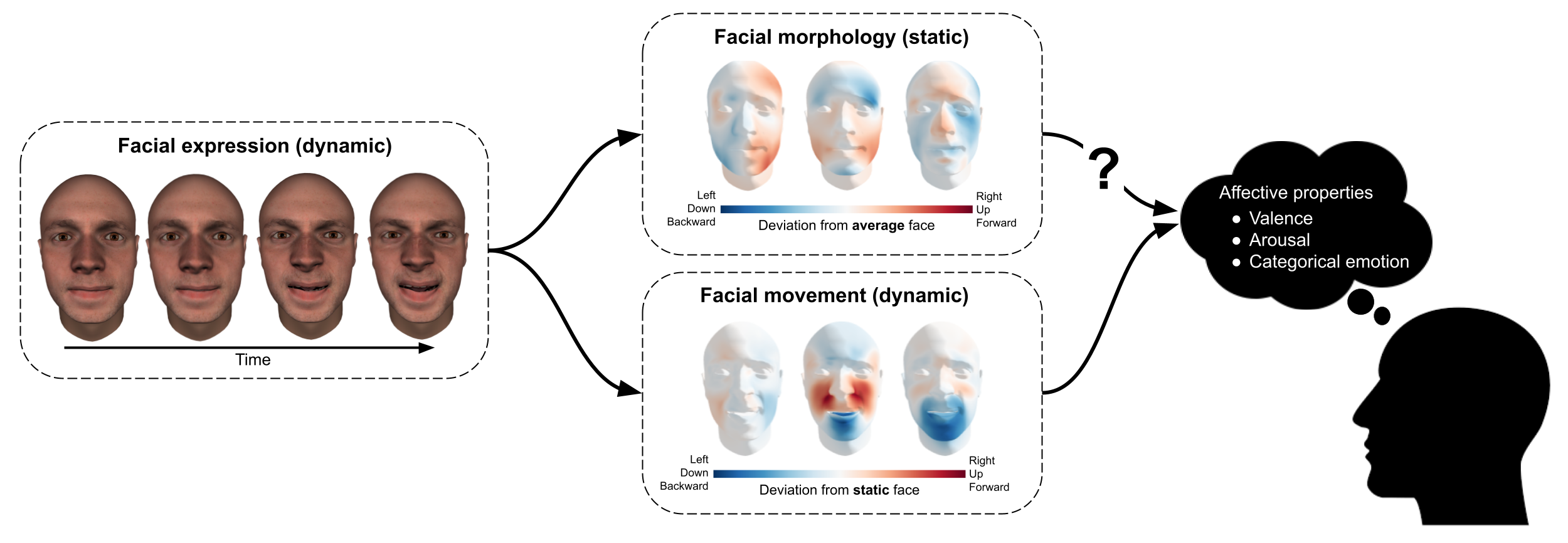
Figure 7.1: Decomposition of facial expressions in static information (facial morphology) and dynamic information (facial movement), where static information is operationalized as shape deviation relative to the average face while dynamic information is operationalized as shape deviation relative to the static face. The current study’s aim is to quantify the importance of static information, relative to dynamic information, in affective perception.

7.2 Methods

7.2.1 Participants

Thirteen participants (7 female, 6 male) participated in the “Facial Expression Encoding and Decoding” project, which consisted of six psychophysics sessions and six (7T) MRI sessions. Participants were recruited through Facebook. With the exception of three participants, all participants were students of the Research Master Psychology or master Brain & Cognitive Sciences at the University of Amsterdam. Several strict exclusion criteria for participation were applied, including standard MRI safety-related exclusion criteria, psychiatric conditions, use of psychopharmacological medication, color blindness, and difficulty with remembering faces. Additionally, participants had to have participated in MRI research before and had to be between 18 and 30 years of age (resulting sample M_age = 22.6, SD_age = 3.7).

Across six psychophysics sessions, participants rated the perceived valence, arousal, and categorical emotion of short clips of dynamic facial expressions. These stimuli were generated using a 3D Morphable Modeling toolbox developed by and described in Yu et al. (2012). The toolbox allows to generate short video clips of facial expressions with a configuration of prespecified “action units” (AUs) that describe particular visually recognizable facial movements. It does so by manipulating the structure of a 3D mesh representing the surface of the face according to the expected deformation in response to the activation of one or more AUs. Apart from amplitude (ranging from 0, inactive, to 1, maximally activated), several temporal parameters corresponding to the AU activation (onset latency, offset latency, acceleration, deceleration, and peak latency) can be manipulated. In the toolbox, AU animations can be applied to any 3D face mesh from a database of 487 different faces (“face identities”), which vary in sex, age, and ethnicity.

For our stimuli, we used 50 different face identities that were restricted to be of Western-Caucasian ethnicity and to an age between 18 and 30 years old (i.e., the same age range as our participants). This set of face identities contained 36 female faces and 14 male faces. To animate each face stimulus, we selected a random subset of AUs from a set of twenty bilateral AUs (AU1, AU2, AU4, AU5, AU6, AU7, AU9, AU10Open, AU11, AU12, AU13, AU14, AU15, AU16Open, AU17, AU20, AU24, AU25, AU27i, AU43). The number of AUs for each stimulus were drawn randomly from a binomial distribution with parameters n = 6 and p = 0.5 (but with a minimum of 1 AU). The amplitude of each AU activation was randomly selected from three equidistant values (0.333, 0.667, and 1). The temporal parameters were the same for each stimulus, which corresponds to a stimulus with a duration of 1.25 seconds and in which each AU activation peaks at 0.7 seconds. Each of the 3D face meshes belonging to a single dynamic stimulus was rendered as a short (2D) video clip with a resolution of 600 × 800 pixels containing 30 frames and a frame rate of 24 frames per second.

7.2.2 Experimental design

In total, 752 unique AU configurations were generated with the parameters described above. This process was done separately for two disjoint sets of AU configurations: one set of 696 configurations functioning as the optimization set (used for model fitting) and one set of 56 configurations functioning as the test set (used for model validation; see Cross-validation section). To minimize correlation between AU variables, the sampling process of the number of AUs and AU amplitudes was iterated 10,000 times and the selection yielding the smallest absolute maximum correlation across all AU pairs was chosen (final \(r = 0.093\)). Then, the AU configurations were randomly allocated to the 50 face identities. To minimize the correlation between face identity and AUs, this random allocation was iterated 10,000 times and the selection yielding the smallest (absolute) maximum correlation across all AU-face identity pairs (final \(r = 0.126\)) was chosen. This counterbalancing process was done separately for the optimization and test set.

7.2.3 Procedure

Each participant completed five psychophysics sessions in which they rated a subset of the facial expression stimuli. In the sixth session, participants rated the 50 static faces (i.e., without AU animations) on their perceived attractiveness, dominance, trustworthiness, valence and arousal. These ratings are not used in the current study. Because the test set trials were repeated three times (to estimate a noise ceiling; see Noise ceiling estimation section), the total number of rated stimuli was (696 + 56 × 3 = ) 864. Originally, three sessions were planned in which participants rated 288 stimuli each. Due to a programming bug, however, all but one of the participants rated (unbeknownst to them) the same 288 stimuli in these three sessions. As such, participants completed two extra sessions in which they rated the remaining stimuli with the exception of the (56 × 2 =) 112 test trials, because the three repetitions needed to estimate the noise ceiling were already obtained in the first three sessions. As such, the total number of stimulus ratings was (288 × 3 + 232 × 2 = ) 1328 (and 864 ratings for the single participant without the accidental session repeats).

In each session, the 288 stimuli (or 232 stimuli in session 4 and 5) were rated on three affective properties: categorical emotion, valence, and arousal. Categorical emotion and valence/arousal were rated on separate trials, so each of the stimuli were presented twice (once for a categorical emotion rating and once for a valence/arousal rating). Stimuli were presented in blocks of 36 trials, in which either categorical emotion or valence/arousal was rated. The trial block’s rating type was chosen randomly.

Each session lasted approximately 1.5 hours, which included breaks (after each rating block), setting up and calibrating the eyetracker (which is not used in the current study), an extensive instruction, and a set of practice trials (only in the first block of each session; 10 categorical emotions and 10 valence/arousal ratings). Participants completed the ratings in a dimly lit room, with their head resting on a chin rest (to minimize head movement for the concurrent eyetracking), positioned 80 centimeters from a full HD (1920 × 1080 pixels) monitor (51 × 28.50 cm) on which the rating task was presented using the software package PsychoPy2 (v1.84; Peirce et al., 2019). Participants used a standard mouse (used with their dominant hand) to submit responses during the rating task.

7.2.3.1 Stimulus presentation

Stimuli were presented on a gray background (RGB: 94, 94, 94). Each trial block started with a cue regarding the affective property that should be rated (categorical emotion or valence/arousal) and was followed by a ten second baseline period presenting a fixation target (a white circle with a diameter of 0.3 degrees visual degree, DVA). Then, each facial expression stimulus was presented for 1.25 seconds (the full duration of the clip). The stimulus was shown at the center of the monitor with a size of 6 × 8 DVA (preserving the aspect ratio of the original clip, i.e., 600 × 800 pixels). The stimulus was followed by an interval of 1 second plus a duration drawn from an exponential distribution (with λ = 1) in which only the fixation target was shown. This interval was followed by the presentation of the rating screen (discussed below). The rating screen was shown until the participant gave a response (mouse click). Another interval followed (which included a fixation target) with a duration of 1 second plus a duration drawn from an exponential distribution (with \(\lambda = 1\)), after which the next stimulus was shown. After all 36 trials of a trial block, another baseline period including a fixation target was shown and was followed by the rating type cue of the next block, which the participant could start by a mouse click. After four trial blocks, participants could take a break if desired.

7.2.3.2 Categorical emotion ratings

For the categorical emotion ratings, participants were instructed to “Judge the faces with regards to the emotion that the face shows, if any” (in Dutch: “Beoordeel de gezichten op de emotie die de gezichten (mogelijk) laten zien”). For each categorical emotion rating, participants were presented with a prompt which included six trapezoids (with the corresponding labels “anger”, “disgust”, “fear”, “happiness”, “sadness”, and “surprise” next to it) and a single circle (with the label “None”) arranged in a circle with equal angles between each of the seven options (i.e., 360/7 degrees; see Figure 7.2). The trapezoids had a length of 7 DVA, the circle had a radius of 1 DVA, and the text labels had a text height of 0.7 DVA; the trapezoids, circle, and text were all white. At the onset of the rating prompt, the mouse cursor appeared in the middle of the screen. Participants were instructed to click on the trapezoid corresponding to the perceived emotion from the previously shown facial expression stimulus. Furthermore, participants were instructed to simultaneously rate the intensity of the emotion, which was linked to the radial position of the mouse click within the trapezoid, where responses closer to the center indicated lower intensity and responses farther away from the center indicated higher intensity. After the participant clicked on the trapezoid, the trapezoid changed color from white to black anywhere between the response and the side of the trapezoid closest to the center (see Figure 2). Whenever the facial expression stimulus did not match any of the six categorical emotion labels (“anger”, “disgust”, “fear”, “happiness”, “sadness”, and “surprise”), participants were instructed to click on the circle above the label “None” (“Geen van allen” in Dutch). There was no intensity rating associated with “None” responses. After a response and the change in color of the selected trapezoid or circle, the rating prompt remained on screen for 0.2 seconds. There was no response time limit for the ratings.

7.2.3.3 Valence/arousal ratings

For the valence and arousal ratings, participants were asked to rate how they experienced each face in terms of arousal (on a scale ranging from “not activated” to “activated”) and valence (on a scale ranging from “unpleasant” to “pleasant”). The instructions explained the valence dimension as follows: “On the pleasant/unpleasant dimension, you should indicate how you experience the faces” (in Dutch: “Met de onprettig/prettig dimensie geef je aan hoe jij de gezichten ervaart”). The instructions explained the arousal dimension as follows: “On the not activated/activated dimension, you indicate how much the face activates you. With ‘activated’, we mean that the face makes you feel alert, energized, and/or tense. With ‘not activated’, we mean that the face makes you feel calm, quiet, and/or relaxed” (in Dutch: “Met de niet geactiveerd/geactiveerd dimensie geef je aan in hoeverre het gezicht jou activeert. Met “geactiveerd” bedoelen we dat het gezicht je alert, energiek, en/of gespannen doet voelen; met “niet geactiveerd” bedoelen we dat het gezicht je kalm, rustig, en/of ontspannen doet voelen”).

Valence and arousal ratings were acquired using a single rating prompt (see Figure 7.2). This prompt included two axes (white lines), a horizontal and a vertical one, of equal length (14 DVA). The horizontal axis represented the arousal axis with negative values indicating low arousal (“Not activated”, or “Niet geactiveerd” in Dutch) and positive values indicating high arousal (“Activated”, or “Geactiveerd” in Dutch). The vertical axis represented the valence axis with positive values indicating positive valence (“Pleasant”, or “Prettig” in Dutch) and negative values indicating negative valence (“Unpleasant”, or “Onprettig” in Dutch). Labels at the ends of the axis lines were white and had a text height of 0.7 DVA. Participants were instructed to indicate the valence and arousal of the previously shown facial expression facial expression stimulus by a single mouse click anywhere within the 2D space. After a response, a white circle (0.3 DVA) appeared at the clicked position for 0.2 seconds, after which the rating prompt disappeared.

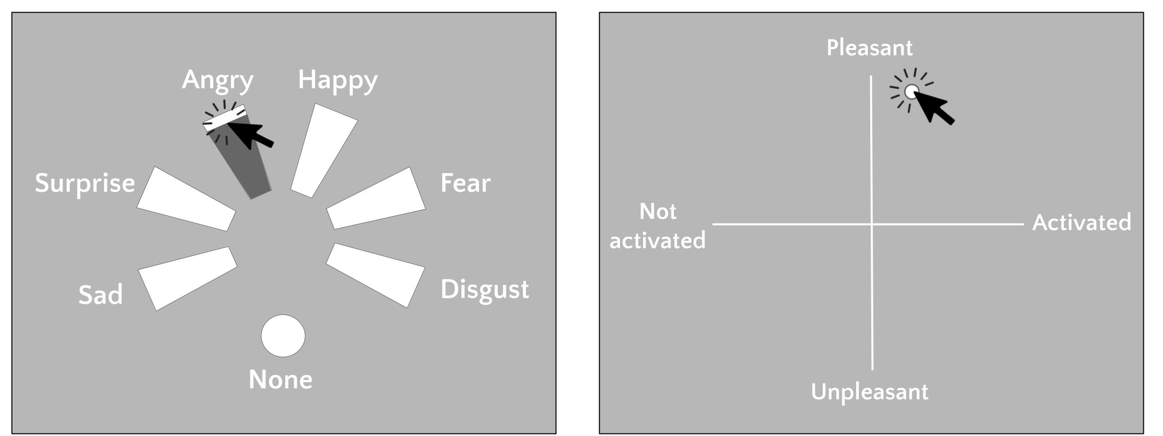
Figure 7.2: Prompts for categorical emotion ratings (left) and valence/arousal ratings (right).

7.2.4 Data preprocessing

7.2.4.1 Rating preprocessing

For the categorical emotion analyses, we removed all ratings in which the participant responded with “None”. This left on average 1125 trials (SD = 165), which is 87% of the total number of trials. The valence and arousal ratings were not filtered or otherwise preprocessed. The accidentally repeated trials from session 1 (that do not belong to the test set; see Cross-validation section) were reduced to a single rating for each unique stimulus by taking the most frequent emotion label (for the categorical emotion ratings) or the average rating value (for the valence/arousal ratings) across repetitions. In addition, the valence and arousal ratings were mean-centered separately for the optimization and test set to correct for spurious differences in the mean across the two partitions.

7.2.4.2 Static and dynamic feature operationalization

As an operationalization of face structure, we use the set of 3D face meshes underlying each dynamic facial expression stimulus. The reason for focusing on the underlying 3D face mesh, instead of the rendered 2D pixel array actually shown to the participants, is that the 3D face mesh allows to isolate face structure information from face texture information while in the 2D pixel space these two factors are confounded. In the 3D face space, each stimulus can be represented as a collection of 30 meshes (corresponding to the 30 frames in each animation), each containing a set of 3D coordinates making up the vertices of the mesh. In our stimulus set, each 3D face mesh has 31049 vertices. As such, any given stimulus can be represented as a 30 (frames) × (vertices) × 3 (coordinates) array with values that represent the position of the vertices in real-world space.

The first step in our feature operationalization pipeline is to separate the static and dynamic information. We operationalize the static information as the 3D face mesh corresponding to the first frame of each stimulus (which corresponds to a “static” or “neutral” face mesh without any AU activation). Using this operationalization, the static information from two stimuli with different AUs (but the same face identity) is equivalent. We operationalize the dynamic information for each stimulus as the difference between the vertex positions at the frame containing the peak AU activation (frame 15) and the first frame. As such, both the static information and the dynamic information of each stimulus can be represented as a 31049 (vertices) × 3 (coordinates) array.

Using all vertex positions as features means that the number of features (i.e., 31049 × 3 = 93147) would vastly outnumber the number of observations (i.e., 752 unique dynamic facial expressions), which makes model fitting prohibitively computationally expensive and bears a high risk of overfitting. As such, reducing the number of features is desirable. The fact that the vertices are highly spatially correlated (i.e., neighboring vertices likely have similar coordinates) warrants using principal component analysis (PCA) to reduce the total feature space. Here, we use PCA to reduce the original feature space (containing 93147 dimensions) to a 50-dimensional space containing variables that represent linear combinations of the original features. Formally, the PCA model estimates a 2D weight matrix, \(W\), with dimensions 50 × 93147 and a mean vector, \(\hat{\mu}\), with length 93147, which are then used to transform the original set of vertices (\(V\); flattened across coordinates) into a 50-dimensional set of features (\(X\)):

\[\begin{equation} X = (V - \hat{\mu})\hat{W}^{T} \end{equation}\]

In this lower-dimensional feature space, almost all variance from the high-dimensional feature space is preserved: about 99.99% for the static feature space and about 99.95% of the dynamic feature space (see Supplementary Figure F.1). The representation of the top four PCA components in vertex space are, for both the static and dynamic feature set separately, visualized in Figure 7.3, which shows that each PCA component represents an interpretable facial movement (e.g., PC1 of the dynamic feature set represents a mouth drop and PC1 of the static feature set represents a relatively wide and long face with a relatively strongly protruding nose and brow).

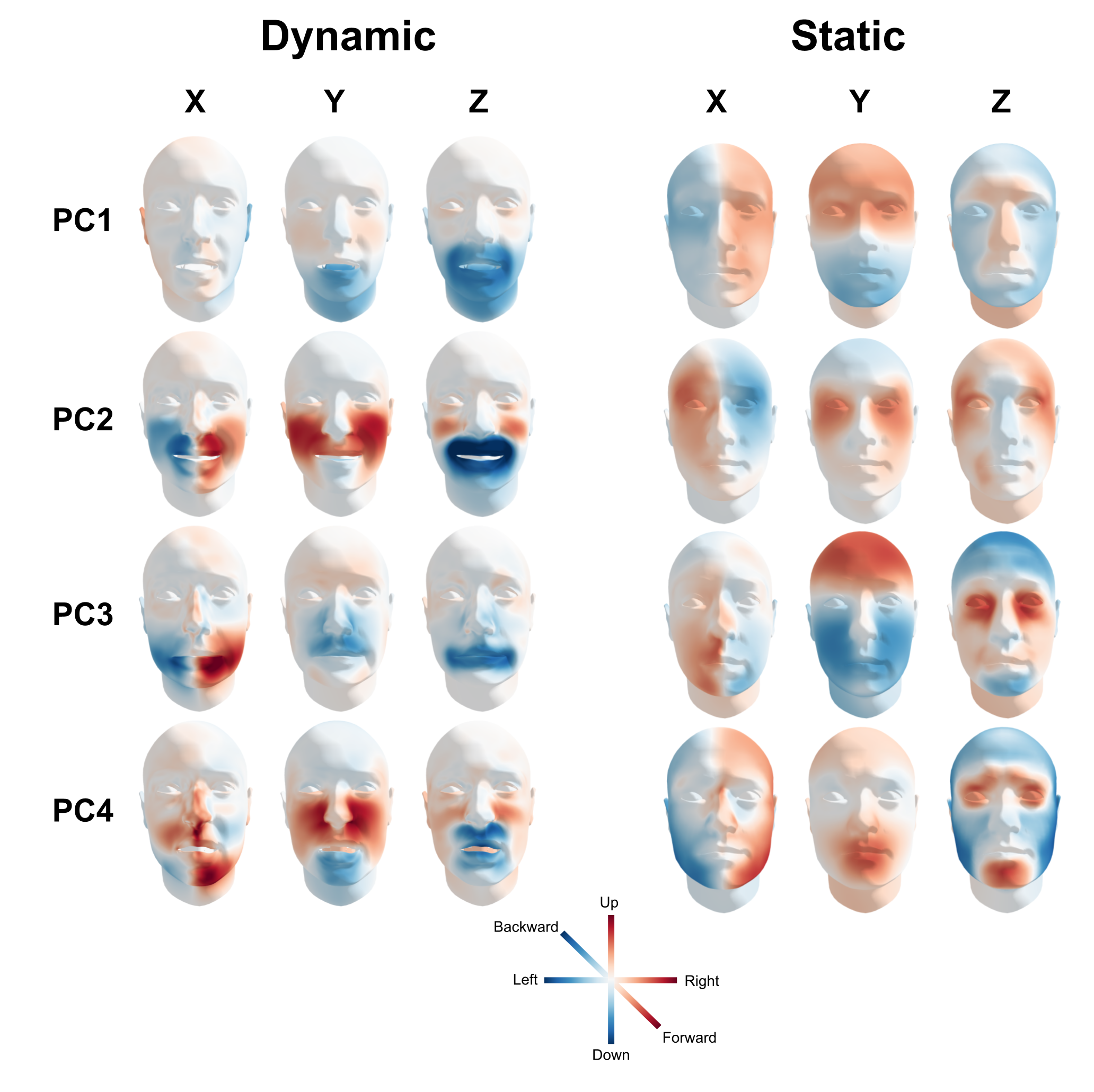
Figure 7.3: Visualization of the extracted PCA components. The first four PCA components of both the dynamic features (left) and static features (right) are visualized by plotting the inverse transform of a single low-dimensional feature set to 3 standard deviations above the average (\(X_{j} := 3\hat{\sigma}_{X_{j}}\)). Colors represent the signed deviation from the mean in standard deviations.

Finally, both the static and dynamic PCA-transformed features (\(X_{j}\)) are divided by their estimated standard deviation (\(\hat{\sigma}_{j}\)) across observations:

\[\begin{equation} X_{j} := \frac{X_{j}}{\hat{\sigma}_{j}} \end{equation}\]

This operation makes sure that each feature has the same scale and thus each feature is equally strongly regularized during model fitting (see Predictive analysis section). Note that usually each feature is additionally mean-centered as well, but this is not necessary because the PCA transform already centers the data.

In the current article, we will refer to a set of PCA-transformed features (\(X\)) as a feature set. In addition to having a dynamic and static feature set, we also horizontally concatenated these two feature sets to create a combined feature set (which thus contains 100 features), which serves to investigate to what extent the two feature sets explain unique variance in the target variables.

7.2.5 Predictive analysis

For our main analysis, we predicted the categorical emotion, valence, and arousal ratings based on static and dynamic features using separate models for each participant. Because the categorical emotion ratings represent a categorical variable, the categorical emotion analysis used a classification model. The valence and arousal ratings represent continuous variables and are therefore analyzed using a regression model. These two types of models are discussed in turn.

7.2.5.1 Categorical emotion model

The categorical emotion analysis used a regularized multinomial logistic regression model as implemented in the Python package scikit-learn (Pedregosa et al., 2011). The choice for this particular predictive model stems from its probabilistic formulation, which makes it suitable for the Bayesian model inversion procedure described in the Bayesian reconstruction section. Formally, the multinomial logistic regression model assumes that the target variable is distributed according to a categorical distribution parameterized as follows:

\[\begin{equation} p(y) \sim \mathrm{Categorical}(g(X\beta + \alpha)) \end{equation}\]

where \(\beta\) represents a set of parameters that are linearly combined with the feature values (\(X\)) and an intercept term (\(\alpha\)), which is passed through the softmax function, \(g\):

\[\begin{equation} g(X_{i}\beta + \alpha) = \frac{e^{X_{ij}\beta + \alpha}}{\sum_{j=1}^{P}e^{X_{ij}\beta + \alpha}} \end{equation}\]

where \(p(y_{i} | X_{i})\) is a vector with a length equal to the number of classes. Although it is possible to derive discrete predictions by subsequently taking the argmax across the vector with class probabilities, we only use the probabilistic predictions because we use a probabilistic model performance metric (Tjur’s pseudo \(R^{2}\); see Performance metrics section). In the context of our categorical emotion analysis, the fitted multinomial logistic regression model outputs predictions in the format of the probability of each of the six categorical emotions given the set of static or dynamic (or their combination) features of a given facial expression stimulus. The logistic regression model was used with balanced class weights to avoid effects due to imbalance across class frequencies, a regularization parameter (C) of 10, and a liblinear solver.

7.2.5.2 Valence and arousal models

Both the valence and arousal analysis used a ridge regression model as implemented in the Python package scikit-learn. Like the multinomial logistic regression model, linear regression models (including the ridge regression model) have a well-defined probabilistic formulation, which assumes that the target variable (\(y_{i}\)) is normally distributed:

\[\begin{equation} p(y) = \mathcal{N}(X\beta, \sigma_{\epsilon}I) \end{equation}\]

where \(~X\beta\) represents the mean and \(\sigma_{\epsilon}I\) the standard deviation of the normal distribution. Note that we do not estimate an intercept term (\(\alpha\)) because we standardize our features (\(X\)) and target variable (\(y\)) before the analysis. After estimating the parameters \(\beta\) and \(\sigma_{\epsilon}\) (i.e., \(\hat{\beta}\) and \(\hat{\sigma}_{\epsilon}\)), predictions for a given observation (\(X_{i}\)) can be made as follows:

\[\begin{equation} \hat{y}_{i} = X_{i}\hat{\beta} \end{equation}\]

In the context of our valence and arousal model, this means that the valence and arousal values are predicted on the basis of a linear combination of the static or dynamic features. The ridge regression model was fitted with a regularization parameter of 500 and without an intercept.

7.2.5.3 Cross-validation procedure

To facilitate optimization of the analysis and model hyperparameters without the risk of overfitting (Kriegeskorte et al., 2009), the data (i.e., all 752 unique stimuli and associated ratings) were divided into two independent sets: an optimization set with 564 unique stimuli and a test set with 150 unique stimuli (which contains 450 ratings, because each test trial was repeated three times in order to estimate a within-participant noise ceiling). Note that the set of unique test set stimuli is composed of the 56 stimuli originally designated as test set stimuli and an additional 96 stimuli randomly sampled from the accidental repeated trials from the first session; the reason to increase the test set size is to reduce the variance in the estimate of model performance (Varoquaux et al., 2017; Varoquaux, 2018). The distribution of categorical emotion, valence, and arousal ratings is visualized, separately for the optimization and test set, in Supplementary Figure F.2, which shows that the two sets are very similar in their rating distributions.

Within the optimization set, we compared different preprocessing techniques (such as standardization before or after PCA fitting) and model hyperparameters (such as the model’s regularization parameter, which was evaluated for \(\alpha\) and \(\frac{1}{C}\): 0.01, 0.1, 1, 10, 50, 100, 500, 1000). This was done using repeated 10-fold cross-validation within the optimization set, which entails fitting the model on 90% of the data (the “train set”) and evaluating the model performance on the prediction of the left out 10% of the data (the “validation set”). The results of this optimization procedure indicated that a regularization parameter of 10 for the logistic regression model and a regularization parameter of 500 for the regression models led to the highest cross-validated model performance within the optimization set, which were used for each participant-specific model.

This cross-validation procedure within the optimization set was repeated multiple times to optimize the preprocessing and model hyperparameters, which results in a positively biased estimate of cross-validated model performance (Kriegeskorte et al., 2009). As such, we fitted each model with the optimal hyperparameters (as reported in the Categorical emotion model and Valence/arousal models sections) once more on the entire optimization set and subsequently cross-validated it to the test set. This cross-validation from the optimization to test set was only done once to ensure an unbiased estimate of cross-validated model performance. Notably, in the test set, the trial repetitions were not reduced to a single rating in order to estimate the noise ceiling specifically for the model performance on the test set.

7.2.5.4 Performance metrics

To evaluate the cross-validated model performance of the categorical emotion model, we used Tjur’s pseudo \(R^{2}\) score (Tjur, 2009). We chose this particular metric instead of more well-known metrics for classification models (such as accuracy) because it is insensitive to class frequency, allows for class-specific scores, and has the same scale and interpretation as the \(R^{2}\) score commonly used for regression models (Dinga et al., 2020). To evaluate the cross-validated model performance of the valence and arousal models, we used the \(R^{2}\) score. Note that the theoretical maximum value of both Tjur’s pseudo \(R^{2}\) score and the regular \(R^{2}\) score is 1, while the minimum of Tjur’s pseudo \(R^{2}\) score is -1 and the minimum for the regular \(R^{2}\) score is unbounded; chance level for both metrics is 0.

7.2.5.5 Population prevalence

Although participant-specific cross-validated model performance scores are unbiased estimates of generalizability, above chance level estimates may be due to chance (although this is unlikely given the relatively large size of our test set; Varoquaux, 2018). Additionally, reporting only summary statistics (such as the mean or median) of the set of within-participant model performance estimates ignores the between-participant variance. One possibility to summarize and quantify model performance across the set of participants is to test their mean score against the theoretical chance level using a one-sample t-test. This approach, however, is invalid for unsigned metrics, such as the (pseudo) \(R^{2}\) scores used in this study, which logically cannot have a population mean below chance level and thus cannot be tested using a one-sample t-test (which assumes a symmetric gaussian sampling distribution around the chance level; Allefeld et al., 2016).

An alternative statistical framework is provided by prevalence inference (Allefeld et al., 2016; Rosenblatt et al., 2014), which estimates the proportion of the population that would show the effect of interest. Here, we use the Bayesian approach to prevalence inference described by Ince et al. (2020). This particular implementation estimates a posterior distribution of the population prevalence proportion (a number between 0 and 1), which is based on the number of statistically significant effects across participants. Statistical significance for a given participant (i.e., the “first-level test statistic”) is computed using a non-parametric permutation test (Allefeld et al., 2016; Ojala & Garriga, 2010), in which the observed cross-validated model performance score is compared to the distribution of model performance scores resulting from the model predictions on permuted test set values. Formally, the p-value corresponding to an observed score, \(sc^{\mathrm{obs}}\), given a set of Q permutation values, \(sc^{\mathrm{perm}}\), is computed as follows:

\[\begin{equation} p = \frac{\sum_{p=1}^{Q} I(sc_{i}^{\mathrm{perm}} \geq sc^{\mathrm{obs}}) + 1}{Q + 1} \end{equation}\]

where \(I\) is an indicator function return 1 when the expression in brackets \((sc_{i}^{\mathrm{perm}} \geq sc^{\mathrm{obs}})\) is true and 0 otherwise. In our analyses, we ran 1000 permutations and used a significance level (\(\alpha\)) of 0.05. Note that although significance of participant-specific effects is computed using a binary decision threshold (as is done in traditional null-hypothesis significance testing), the posterior resulting from the Bayesian prevalence inference analysis is not thresholded.

The issues associated with group-level tests of model performance against chance level do not apply to group-level tests between model performance estimates of different classes of the target variable (e.g., between different emotions), because a symmetric distribution can be assumed for these values.

7.2.6 Noise ceiling estimation

If there is measurement noise in the target variable, perfect model performance (i.e., at the theoretical maximum) is impossible. In case of measurement noise, it is more insightful to compare model performance to an estimate of the noise ceiling, an upper bound that is adjusted for measurement noise in the target variable (Lage-Castellanos et al., 2019). We developed a method to derive noise ceilings for classification models, which is reported and explained in detail in Chapter 7. We use this method to estimate noise ceilings for our categorical emotion models.

For the valence and arousal models, we developed a method to estimate a noise ceiling, assuming that the regular \(R^{2}\) score is used, that is very similar to the aforementioned method to estimate noise ceilings for classification models (see for a related method, Sahani & Linden, 2003; Schoppe et al., 2016). Recall that the \(R^{2}\) score is computed as 1 minus the ratio of the residual sum of squares (RSS) to the total sums of squares (TSS):

\[\begin{equation} R^{2} = 1 - \frac{RSS}{TSS} = 1 - \frac{\sum_{i = 1}^{n}(y_{i} - \hat{y}_{i})^{2}}{\sum_{i = 1}^{n}(y_{i} - \bar{y}_{i})^{2}} \end{equation}\]

where the RSS term is the sum of the squared deviations of the predicted values (\(\hat{y}_{i}\)) from the true values (\(y_{i}\)) of the target variable. The \(R^{2}\) noise ceiling can be computed using the previous formula when setting the prediction of each unique observation to the mean across its repetitions, which represents the optimal prediction any regression model can make given the variance across repetitions. Formally, for observation \(i\) repeated \(R\) times, the optimal prediction (\(y_{i}^{*}\)) is computed as follows:

\[\begin{equation} y_{i}^{*} = \frac{1}{R}\sum_{r=1}^{R}y_{ir} \end{equation}\]

This formulation follows from the fact that regression models must make the exact same predictions for repeated observations and the prediction that minimizes the residual sum of squares for any given observation is the mean across its repetitions. Note that the computation of the \(R^{2}\) noise ceiling does not depend on the actual model used for prediction, but only on the design matrix (\(X\), which determines which observations are repetitions) and the target variable (\(y\)). It follows that for a target variable without repeated observations, the \(R^{2}\) noise ceiling is 1. For more details on the conceptual and mathematical basis of this method, see Snoek et al. (n.d.).

7.2.7 Bayesian reconstructions

The predictive analyses in the current study predict the affective property (\(y\)) given a set of static or dynamic features (\(X\)), with the aim to approximate the process underlying affective face perception. Another, complementary goal might be to estimate and visualize, or “reconstruct”, the features (\(X\)) that underlie a particular affective percept (\(y\)), as is commonly done in reverse correlation studies (Brinkman et al., 2017; Jack & Schyns, 2015, 2017). Usually, such reverse correlation studies estimate the relationship between stimulus features (\(X\)) and the target variable (\(y\)) separately for each feature and (in case of a categorical target variable) different classes of the target variable. Although this strictly univariate approach has yielded valuable insights across various scientific domains including vision (Neri et al., 1999), neuroscience (Ringach & Shapley, 2004), and more recently, social psychology (Brinkman et al., 2017), we believe it can be improved in terms of parsimony and flexibility. First, univariate correlation methods assume that each feature (\(X_{j}\)) is independent from all other features. This assumption may hold for stimulus sets that are completely randomly generated, but for stimuli that are parameterized by more complex and correlated features (such as facial movements), this assumption may break down. Furthermore, typical reverse correlation methods yield point estimates of the relationship between features and the target variable (usually correlations), which ignores the uncertainty of the resulting feature space visualizations.

To overcome these limitations, we use a multivariate Bayesian version of reverse correlation to reconstruct the typical dynamic and static features underlying categorical emotions and valence and arousal levels. This technique is increasingly popular in systems neuroscience (Bergen et al., 2015; Naselaris et al., 2011; Wu et al., 2006), where it is used to reconstruct stimulus features (such as the stimulus orientation) or complete stimuli (i.e., their pixel values) from neural data. This approach consists of two steps. First, an encoding (or forward) model is estimated, which predicts the neural data as a (usually linear) function of the stimulus features. Second, using Bayes theorem, the encoding model is “inverted” to generate a reconstruction (or backward) model that estimates the stimulus features for a given pattern of neural data. Formally, for a given encoding model estimating the probability of the target variable given a set of stimulus features, \(p(y | X)\) (i.e., the likelihood), the reconstruction model, \(p(X | y)\) (i.e., the posterior) can be obtained as follows:

\[\begin{equation} p(X | y) = \frac{p(y | X)p(X)}{p(y)} \end{equation}\]

where \(p(X)\) represents the prior distribution on the stimulus features and \(p(y)\) represents a normalizing constant. Importantly, in this inversion step, the previously estimated parameters of the encoding model (e.g., \(\hat{\beta}\), \(\hat{\alpha}\), and \(\hat{\sigma}_{\epsilon}\) in a typical logistic or linear regression model) are fixed. In the context of the current study, the encoding models are the logistic and linear regression models that predict the target variable (categorical emotion, valence, and arousal) as a linear function of dynamic or static stimulus features. The reconstructions shown in the results section are based on the parameters (\(\hat{\beta}\), \(\hat{\alpha}\), and \(\hat{\sigma}_{\epsilon}\)) averaged across all participant-specific encoding models.¹⁹

In our reconstructions, we estimate the most probable stimulus given a particular value of the target variable, \(p(X | y)\). For our categorical emotion reconstructions, we reconstruct the most probable face for each of the six categorical emotions separately; for the valence and arousal models, we reconstruct the most probable face at seven different levels of the target variable: -0.6, -0.4, -0.2, 0.0, +0.2, +0.4, and +0.6. These target values are on the same scale as the original ratings (which ranges from -1 to 1). Importantly, these values represent the ratings before normalization such that a value of 0 represents the midpoint of the scale. We do not reconstruct the faces corresponding to the extremes of the scales (i.e., between -0.6 and -1 and +0.6 and +1), because the models rarely make predictions of this magnitude (see Supplementary Figure F.5) and as consequence such reconstructions tend to yield morphologically unrealistic faces.

To not bias the reconstructions to a particular configuration, we use a uniform prior on the stimulus features, bounded by the minimum and maximum values observed in our PCA features (\(X\)), which ensures that the reconstructions do not include morphologically implausible configurations:

\[\begin{equation} p(X_{j}) = U(\min(X_{j}), \max(X_{j})) \end{equation}\]

Because the denominator in Bayes formula is often not possible to derive analytically, we estimate the posterior distribution using Markov Chain Monte Carlo (MCMC) sampling as implemented in the Python package pymc3 (Salvatier et al., 2016). We used the package’s default sampler (NUTS) with four independent chains, each sampling 10,000 draws (in addition to 1000 tuning draws) from the posterior. In the current study, the posterior distribution for each feature represents the probability of the value of each dynamic or static stimulus feature for a given categorical emotion or valence or arousal value. For our reconstructions, we estimate the most plausible reconstruction from the posterior. Instead of using the model’s maximum a posteriori (MAP) values (which often fail to coincide with the region of highest density in high-dimensional posteriors; Betancourt, 2017), we use the midpoint between the bounds of the 5% highest posterior density interval (HDI):

\[\begin{equation} X_{j}^{*} = \frac{1}{2}(\mathrm{HDI}(X_{j})_{\mathrm{upper}} - \mathrm{HDI}(X_{j})_{\mathrm{lower}}) \end{equation}\]

The posteriors and chosen reconstruction values for the first ten features (\(X_{1}-X_{10}\)) are visualized in Supplementary Figure F.6 (for the dynamic feature set) and Supplementary Figure F.7 (for the static feature set), which shows that our chosen reconstruction values correspond to the posterior’s point of highest density. From this figure, one particular limitation with respect to the inversion of the categorical emotion model becomes clear, i.e., that most posteriors peak at the extremes of the corresponding feature values. The reason for this is that the softmax function maps values (i.e., \(X\)) from an arbitrary scale to the 0-1 domain (i.e., \(p(y | X)\)) and cannot be inverted to yield the exact feature values (i.e., \(X^{*}\)) given a particular probability; in fact, for a given probability, the “inverted softmax” can yield infinitely many different possible feature value combinations (\(X^{*}\)), but because of the target (\(y\)) follows a multinomial distribution (with \(p = \mathrm{softmax}(X\beta+\alpha)\)), the probability of each feature value increases proportionally to its magnitude. However, this issue does not affect the relative differences in magnitude between feature values (e.g., \(X_{j}^{*}\) is twice as large as \(X_{j+1}^{*}\)) and thus does not affect the quality of the reconstructions.

In the current study, the values of the posterior represent the PCA-transformed variables. To transfer these values into vertex-space, we need to invert the standardization step and the PCA-transform as well, which involves the following linear transformation from PCA-space (\(X_{*}\)) to vertex-space (\(V^{*}\)):

\[\begin{equation} V^{*} = (X^{*}\hat{\sigma})\hat{W} + \hat{\mu} \end{equation}\]

where \(V^{*}\) represents the most probable static face or most probably dynamic movement in vertex-space (i.e., a 31049 × 3 array) given a particular emotion or valence/arousal value (see Figure 7.4 for a visualization of the reconstruction procedure). Notably, unlike traditional univariate reverse correlation reconstructions, the reconstruction values from the Bayesian approach discussed here are in the original units of the feature space (here: vertex positions or deviations) and are thus directly interpretable and can be visualized in a straightforward manner.

To interpret and gain further insight into the (relations between the) reconstructions, we visualize the dynamic movements on top of the average static face and for both the static and dynamic information reconstructions. We color-code the deviations separately for the X, Y, and Z dimension. In these visualizations, blue colors represent leftward (X), downward (Y), or backward (Z) deviations/movements and red colors represent rightward (X), upward (Y), or forward (Z) deviations/movements. The software package plotly (https://plotly.com/python) was used to create the visualizations. Moreover, to gain insight into how different reconstructions relate to each other (e.g., across different emotions or across static and dynamic reconstructions for a given affective attribute), we compute the Pearson correlation between any two reconstructions (flattened across spatial coordinates into a vector of length 93147).

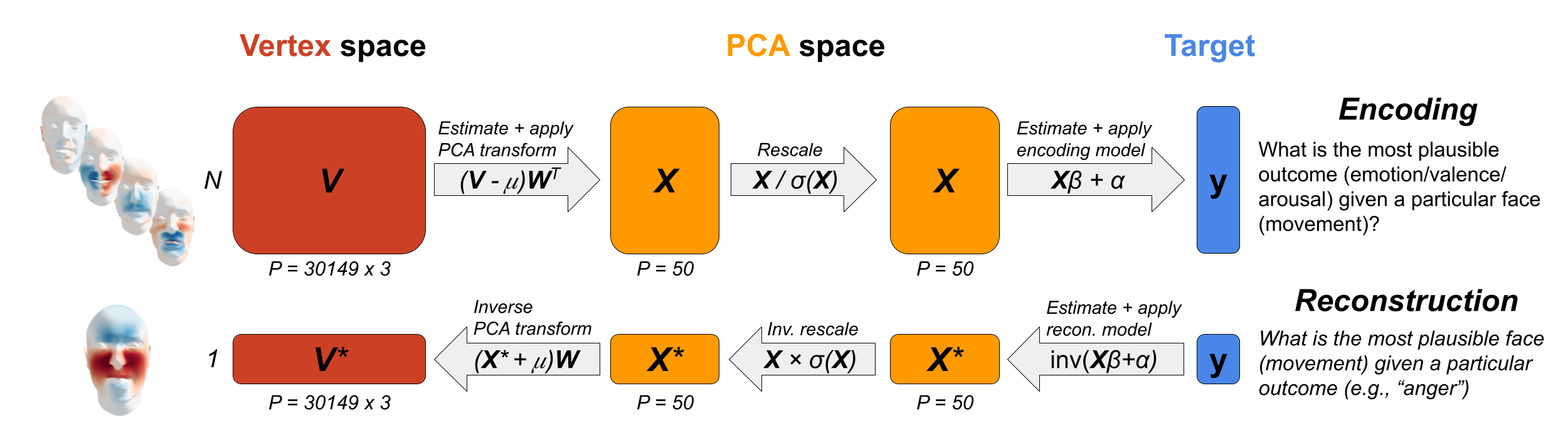
Figure 7.4: Visualization of the encoding (“forward”) model (top) and the reconstruction (“backward”) model (bottom). Note that during the encoding step, a set of \(N\) observations is used to estimate the parameters of the encoding model, while in the reconstruction step only a single observation is reconstructed (although reconstruction can be done for multiple observations at once, if desired).

7.2.8 Code availability

All code used for the analyses reported in the current study are available on Github: https://github.com/lukassnoek/static-vs-dynamic. Additionally, code to estimate noise ceilings for both classification and regression models has been released as a Python package, available on Github: https://github.com/lukassnoek/noiseceiling. The code used for this project makes frequent use of the Python packages numpy (Harris et al., 2020), pandas (McKinney & Others, 2011), scikit-learn (Pedregosa et al., 2011), matplotlib (Hunter, 2007), and seaborn (Waskom, 2021). The prevalence inference estimates were computed using the bayesprev Python module from Ince et al. (2020).

7.3 Results

In the next two subsections, we report the model performance of the encoding model and the reconstructions from the reconstruction model.

7.3.1 Encoding model performance

Figure 7.5 summarizes the average explained variance for each affective property (and, in the context of the categorical emotion analysis, different emotions), separately for the static, dynamic, and combined feature sets. For all affective properties, the model based on the combined feature set explains approximately as much as the sum of the static and dynamic model performance (see Supplementary Figure F.4, indicating that static and dynamic features explain unique and additive variance. Moreover, the general pattern of results is very similar to (and thus replicates) the results obtained on the optimization set (see Supplementary Figure F.3. The posteriors of the population prevalence estimates associated with the model performance scores are visualized in Figure 7.6.

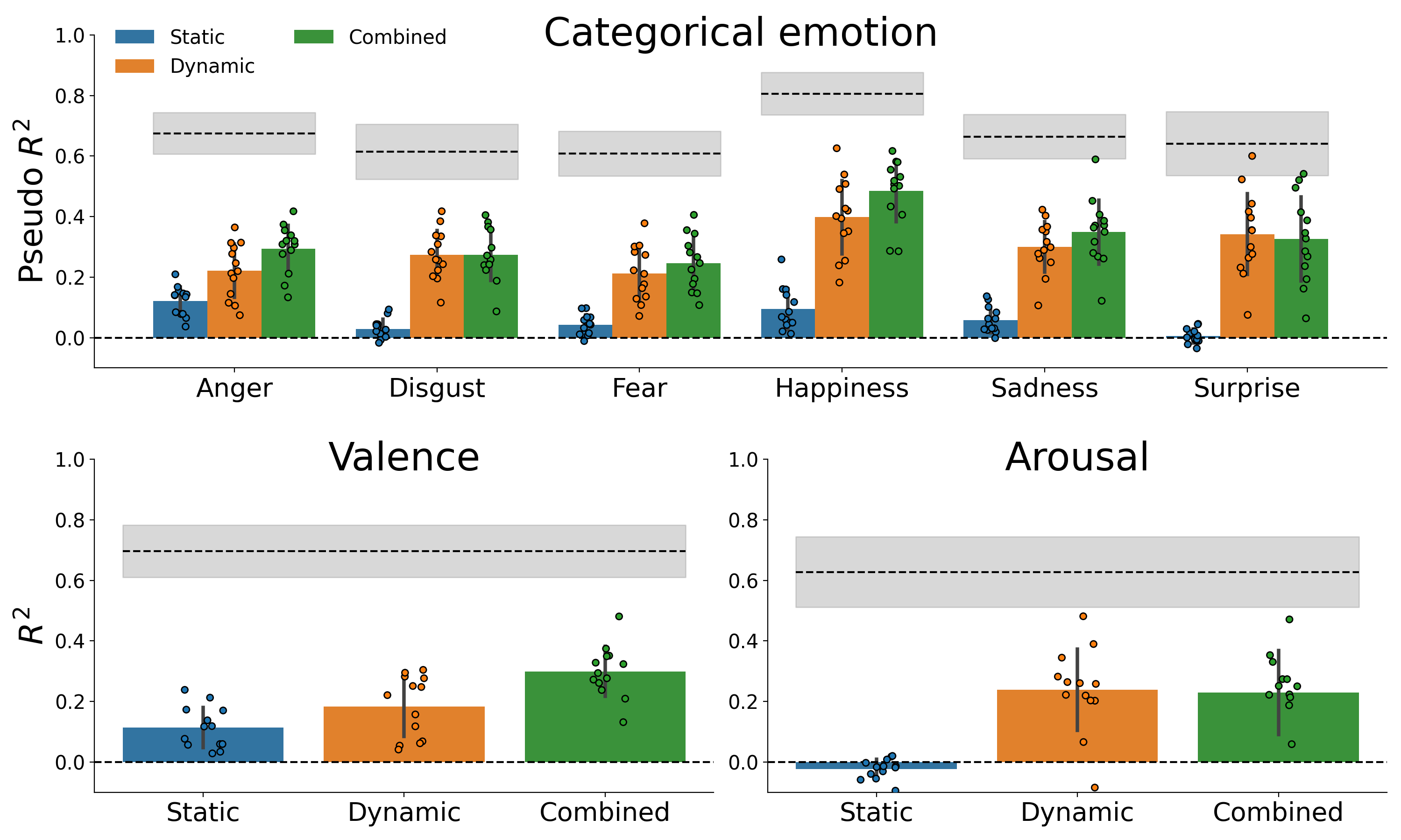
Figure 7.5: Cross-validated model performance, shown separately for each target feature (top: categorical emotion, bottom left: valence, bottom right: arousal) and feature set (static, dynamic, and combined). The bar height represents the mean model performance across participants and the error bars represent ±1 SD. The average within-participant noise ceiling of the combined feature set is plotted for reference as a dashed black line, which is surrounded by a grey area indicating ±1 SD.

7.3.1.1 Categorical emotion model

In the categorical emotion analysis, on average about 5.8% of the variance can be explained by static features (versus 29.1% by dynamic features and 33.1% by the combined feature set). The highest percentages explained variance per emotion were observed for anger (12.1%) and happiness (9.4%), which were significantly higher than the percentages for the other emotions (evaluated using a paired samples t-test, all p < 0.05). The magnitude of the average cross-validated pseudo \(R^2\) scores is roughly proportional to the expected proportion of the population to show an effect (i.e., a cross-validated pseudo \(R^{2}\) significantly larger than 0), as is shown in Figure 7.6. The population prevalence estimates across emotions range from 23% (for surprise) to 100% (for anger). For the dynamic and combined model, an effect is expected in the entire population (i.e., a population prevalence of 100%).

7.3.1.2 Valence/arousal models

Relative to the averaged predictive power of the static features for the categorical emotion model, the predictive power of static features is higher in the valence model, in which it explains on average 11.4% of the variance (versus 18.3% using dynamic features and 30.0% using the combined feature set). This is substantially lower in the arousal model, in which negative \(R^{2}\) values are observed when using static features (versus 23.9% using dynamic features and 22.9% using the combined feature set). The computed population prevalence estimates confirm that a statistically significant effect is expected in virtually the entire population for all valence and arousal models, with the exception of the static arousal model, in which an effect is only expected in 30% of the population).

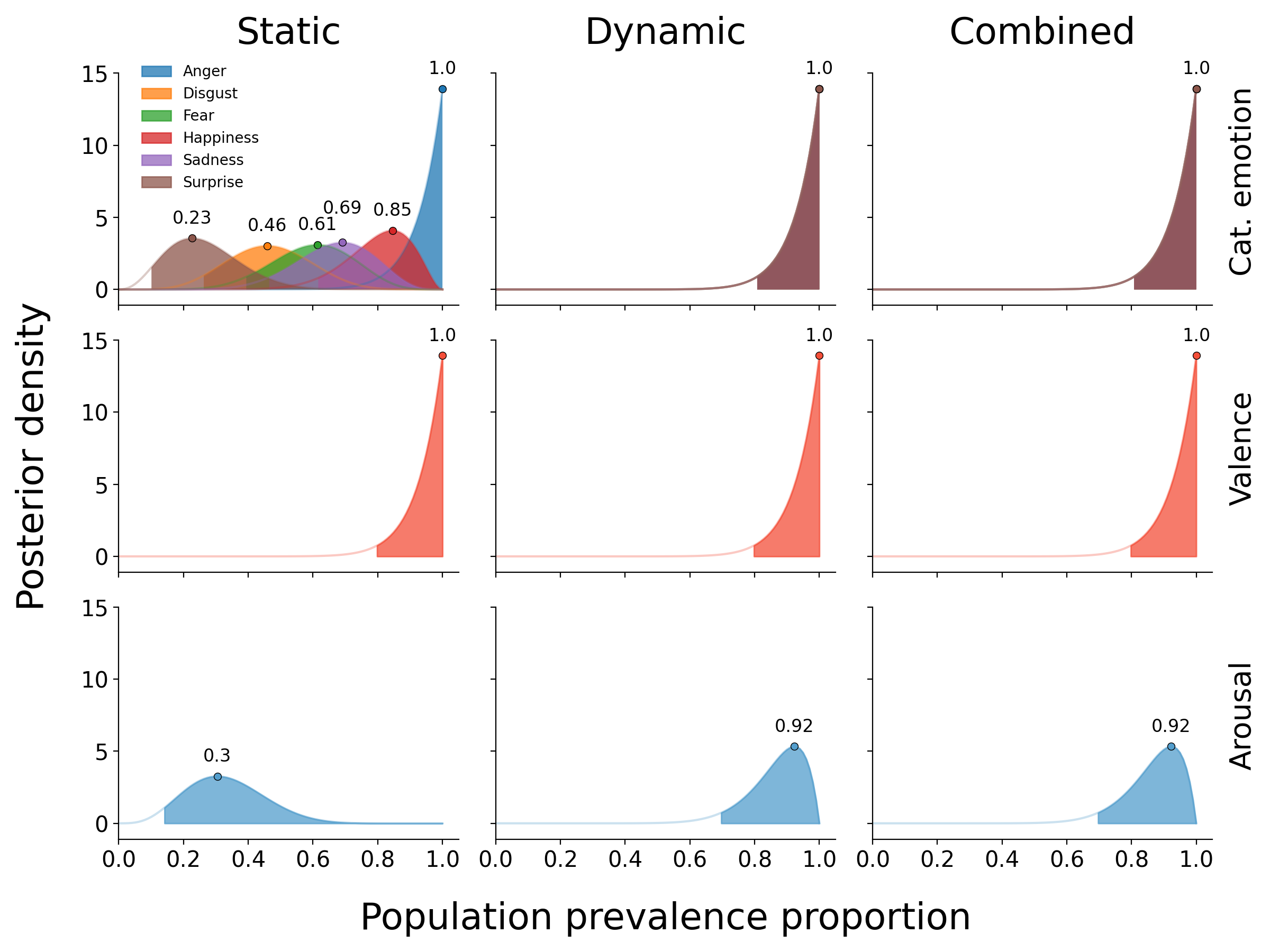
Figure 7.6: The posterior distributions for the population prevalence proportion of the results from the categorical emotion (top), valence (middle), and arousal models (bottom). The posteriors for the different emotions with respect to the dynamic and combined categorical emotion model performances completely overlap, so only a single posterior is shown. The filled area represents the probability density higher than the lower bound of the 96% highest density interval (McElreath, 2020).

7.3.2 Reconstruction model visualizations

Using the estimated coefficients from the encoding models, we estimated the most likely dynamic and static stimulus features for a given categorical emotion or valence/arousal level. In Figure 7.7, we visualize these reconstructions.

7.3.2.1 Categorical emotion reconstructions

Based on a qualitative visual assessment, the reconstructions from the categorical emotion model based on dynamic information conform to the stereotypical facial expressions associated with categorical emotions (cf. Ekman et al., 1969; Jack et al., 2016). As can be seen in Figure 7.8, anger is associated with a jaw drop, narrowing of the face, raised cheeks, and a lowered brow; disgust is associated with a raised upper lip, raised cheeks, and tightened eyelids; fear is associated with a strong jaw drop and brow raise; happiness is associated with a raised cheeks (which also widens the face), tightened eyelids, and slightly raised eyebrows; sadness is associated with pressed lips, widening of the cheeks, and closed eyes; and surprise is associated with a jaw drop, narrowing of the face and raised eyebrows. Although no stereotypical face structures have been proposed in the literature, the majority of the static reconstructions still show clear and interpretable facial features for most categorical emotions. Anger is associated with a relatively wide face, high forehead, and a protruding nose and chin; disgust is associated with an asymmetric face (in the left-right direction) and protruding mouth/lips; fear is associated with a relatively narrow face and turned-up nose, and slightly protruding mouth; happiness is associated with turned-up mouth corners and high cheekbones; and sadness is associated with a relatively long face and protruding eyebrows. We retrain from interpreting the reconstruction of the static surprise face because static features were not found to be predictive for surprise (see Figure 7.5).

In addition to qualitatively assessing the reconstructions separately, we also compared them quantitatively to each other. In Figure 7.8 (top left), we visualize the correlation matrix of the dynamic categorical emotion reconstructions. This correlation matrix shows relatively high correlations between reconstructions of “anger” and “disgust” (\(r = .62\)) as well as “surprise” and “fear” (\(r = .56\)), which may underlie the relative frequent confusion between those pairs of emotions (see Supplementary Figure F.5, top left). The correlation matrix of the static categorical emotion reconstructions (Figure 9, middle left), in contrast, shows no clear similarities across reconstructions. Finally, we computed the correlation (for each emotion pair) between the static and dynamic reconstructions, which indicates the extent to which static and dynamic share the same “face topology”. If dynamic and static reconstructions are in fact similar in terms of face topology, we would expect high values on the diagonal of the matrix and low values elsewhere. This actual correlation matrix (Figure 7.8, bottom left), however, does not show this pattern; all correlations between the dynamic and static reconstructions are around 0.

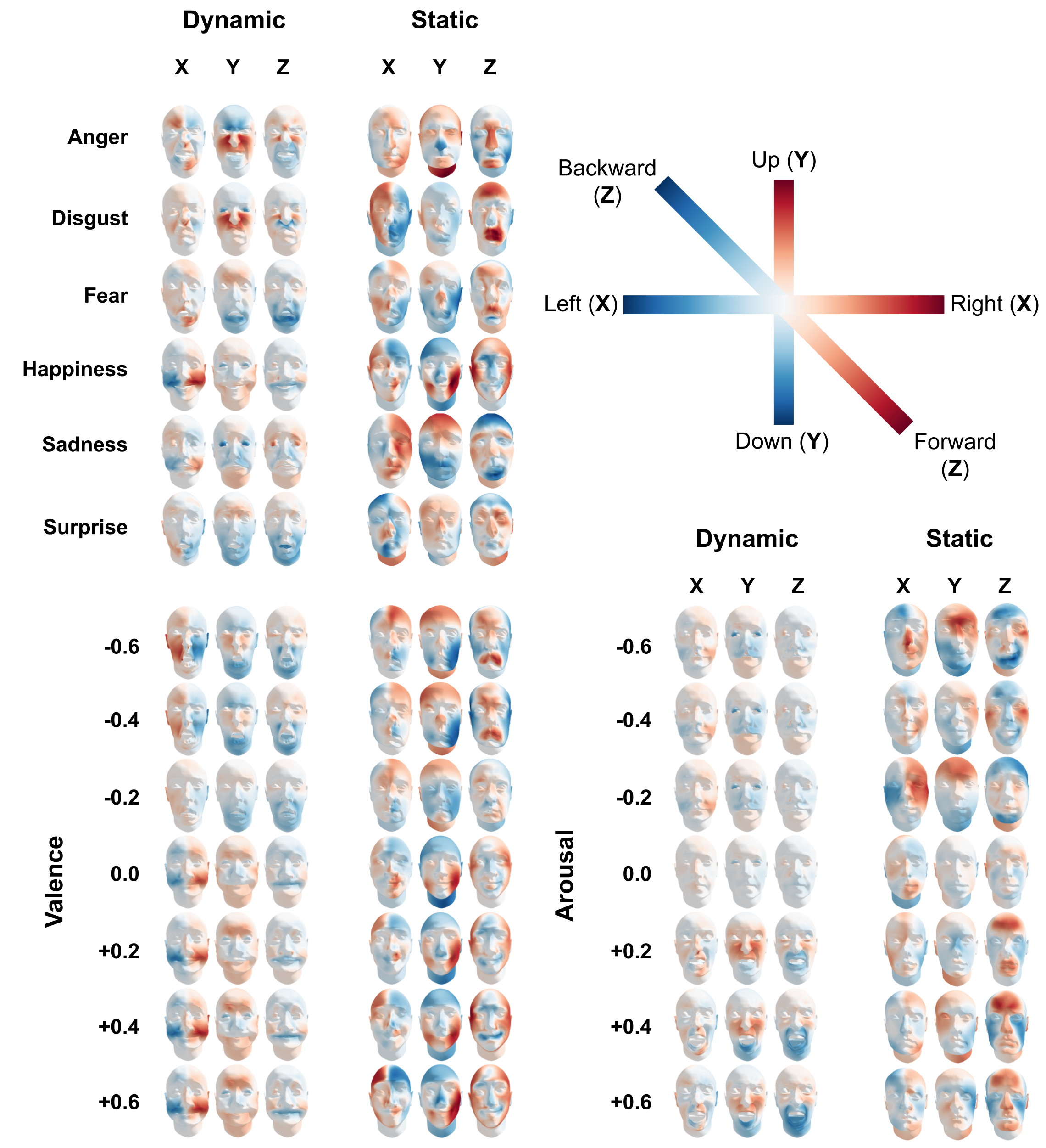
Figure 7.7: The results from the Bayesian reconstruction approach for each emotion from the categorical emotion model and for seven levels, -0.6, -0.4, -0.2, 0, +0.2, +0.4, and +0.6, of the valence and arousal model, shown separately for the static and dynamic feature sets. Color saturation is proportional to the movement or deviation in vertex space (in SD).

7.3.2.2 Valence/arousal reconstructions

The reconstructions from the dynamic valence model also show clear facial movements for both highly negative and highly positive valence values. A face that is experienced as highly negative is associated with an “inward” jaw drop, narrowing of the face, and raised cheeks, while a face that is experienced as highly positive is associated with a widening of the face through the cheeks and a raised brow. The reconstructions from the model based on static information shows that faces experienced as highly negative have a wide (“strong”) jawline, a relatively long face, wide forehead, and a protruding brow and mouth, while faces experienced as highly positive have a relatively narrow and short forehead, high cheekbones and mouth corners, and a relatively “flat” face (i.e., positive deviations in the Z dimension at the edges of the face).

The reconstructions from the arousal model based on dynamic information show that faces eliciting low arousal are associated with a widening of the face, tightening of the lips, and tightened/closed eyes, while faces eliciting high arousal are associated with a strong jaw drop, widening of the eyes, and raised cheeks. The reconstructions from the arousal model based on static information, on the other hand, show less interpretable facial features, which is expected based on the low (below-chance) model performance of the static arousal model.

As can be seen in figure 7.7, the reconstructed faces are highly similar across different magnitudes of valence and arousal, respectively. A strongly positive reconstruction, for example, looks almost the same as a weakly positive one. This suggests that the mental representations of these variables seems to be “binary”, even though the variables were measured on a continuous (bipolar) scale and the distribution of the ratings is far from binary (see Supplementary Figure F.2). Moreover, the “switching point” (corresponding to a neutral mental representation) is in some cases offset compared to the midpoint of the rating scale (corresponding to a neutral rating), suggesting a discrepancy between the neutral point of the rating scale and people’s mental representation of a “neutral” face. Note that this phenomenon is less clearly present in the static arousal reconstructions, but given that the static information was not predictive of arousal ratings, we refrain from interpreting these results.

Finally, given the uniformly low correlation values in the cross-correlation matrix between dynamic and static reconstructions of both valence and arousal (Figure 7.8, bottom center and bottom right), it can be concluded that there does not seem to be any correspondence in face topology between static and dynamic representations of valence and arousal.

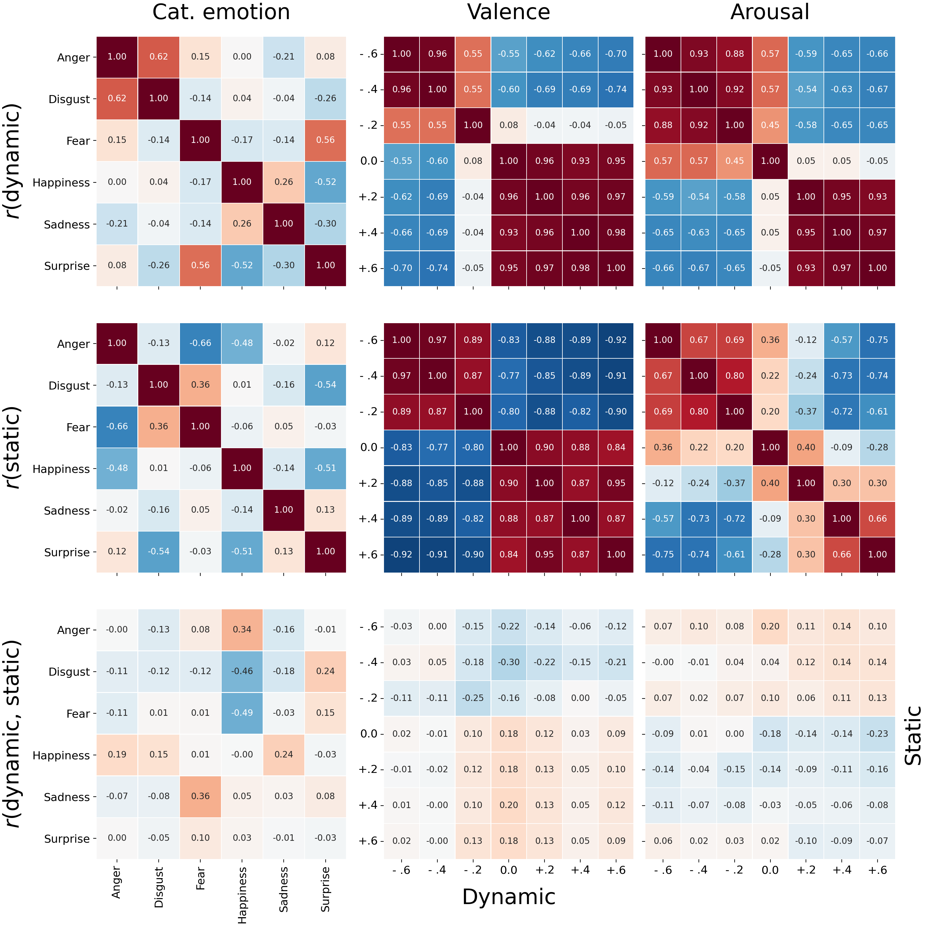
Figure 7.8: Correlations between reconstructions in vertex space for the categorical emotion (left), valence (middle), and arousal (right) models. The top row shows the correlations across all dynamic reconstructions. The middle row shows the correlations across all static reconstructions. The bottom row shows the correlations across each combination of a single dynamic and static reconstruction (e.g., in the bottom left correlation matrix, the top right cell represents the correlation between the static anger and the dynamic surprise reconstruction).

7.3.2.3 Correlations between affective properties

Finally, we evaluated the cross-correlations between the reconstructions of different affective properties. In other words, we evaluate correlations between the reconstructions for different levels of experienced valence and arousal in the observer with the reconstructions for perceived emotions in the face of the expressor (e.g., anger). The correlation matrix of the dynamic reconstruction correlations are visualized in Supplementary Figure F.8 and the correlation matrix of the static reconstruction correlations are visualized in Supplementary Figure F.9. In these correlation matrices, a clear pattern emerged. Specifically, positive valence reconstructions correlated positively with happiness and negative valence reconstructions correlated positively with negative categorical emotion reconstructions (anger, disgust, and fear). Also, low arousal reconstructions correlated positively with happiness and sadness and high arousal reconstructions correlated positively with negative categorical emotion reconstructions (anger, disgust, and fear). Notably, this pattern is both present in the dynamic reconstructions (Supplementary Figure F.8) and static reconstruction (Supplementary Figure F.9). These findings may explain the previously discussed observations that valence and arousal reconstructions seem to be binary instead of graded. Participants may experience a face as categorically positive when a face displays happiness and as categorically negative when a face displays anger, disgust, or fear. Similarly, participants may experience a face as categorically highly arousing when a face displays anger, disgust, or fear and as categorically low arousing when a face displays happiness or sadness.

7.4 Discussion

In the current study, we sought to quantify and disentangle the importance of dynamic features (facial movement) and static features (facial morphology) on affective face perception. Specifically, using machine learning models based on either dynamic features, static features, or a combination thereof, we aimed to predict categorical emotion, valence, and arousal ratings from a psychophysics experiment with dynamic facial expression stimuli that randomly varied in both their facial movements and facial morphology. To gain further insight into the facial features that are important for prediction of the investigated affective properties, we reconstructed the mental representation of faces associated with the different categorical emotions and different levels of experienced valence and arousal using a multivariate reverse correlation method. In what follows, we discuss the current study’s main findings and how they may inform and complement studies on affective face perception.

7.4.1 Facial morphology independently contributes to affective face perception

Our models were able to predict human ratings of perceived categorical emotions and elicited valence substantially above chance level using both dynamic and static features. This demonstrates that not only dynamic but also static features of the face determine in what way people perceive and are affected by facial expressions. Moreover, the sum of the dynamic and static model performance scores approximately equals the combined model performance score for all affective properties, which further indicates that the static and dynamic feature sets carry independent information that is integrated during perception.

The findings of this study have both fundamental and practical implications for (research on) affective face perception. In general, this study shows that the way we perceive and are affected by faces goes beyond what those faces explicitly communicate. Because static features are by definition unrelated to the expressor’s affective state or intentions, one way to frame our findings is that people are biased by features related to facial morphology, perhaps mediated by stereotypes associated with certain demographic groups (e.g., males are thought to display anger more frequently than women; Brooks et al., 2018). In contrast to this interpretation, this “bias” could in fact reflect a true association between morphological features and the frequency of particular affective expressions (e.g., categorical emotions) or predispositions (e.g., dominance; Zebrowitz, 2017). For example, research has shown that facial width-to-height ratio (FWHR) is associated with aggressive behavior (Lefevre et al., 2014), which may mediate the relationship between FHWH and anger perception (see Figure 7.7; Deska et al., 2018). As this debate about the accuracy of the association between facial morphology and affective predispositions is far from solved (see e.g., Jaeger, Oud, et al., 2020; Jaeger, Sleegers, et al., 2020), we leave speculation about this topic to future research that more directly investigates this issue.

On a more practical level, because both static and dynamic features contribute independently to the perception of categorical emotion and experience of valence, researchers studying categorical emotion or valence should use dynamic stimuli of facial expressions instead of static stimuli (i.e., images), which is most commonly done (Krumhuber et al., 2013). By using dynamic stimuli, possible effects of static features can be controlled or explicitly adjusted for. This “decorrelation” of static and dynamic information is important if one wants to say something about the (unconfounded) effect of static or dynamic information in affective face perception. Given our results, dynamic stimuli are also likely to be more effective for eliciting and modelling arousal, which is in line with previous studies that show that arousal is experienced more intensely in response to dynamic than static stimuli (Sato & Yoshikawa, 2007).

7.4.2 The influence of facial morphology does not result from visual similarity to facial movements

Contrary to what is often reported in previous studies (Hess, Adams, & Kleck, 2009; Said et al., 2009; Zebrowitz, 2017), we do not find that static and dynamic features visually resemble each other, as is evident from the low correlations between static and dynamic reconstructions for each categorical emotion and valence and arousal levels. Instead, the static reconstructions show qualitatively different facial features for each emotion and valence/arousal level relative to the dynamic reconstructions. For example, the static anger reconstruction shows a relatively strong jawline (cf. Deska et al., 2018), high forehead, and protruding nose and chin, while the dynamic anger reconstruction shows a narrowing of the face, raised cheeks, and lowered brow. Many of the facial features associated with static reconstructions are similar to facial features associated with social judgments. For example, the strong jawline we observe in the static anger reconstruction has been associated with the perception of dominance (Mileva et al., 2014; Windhager et al., 2011) and the pronounced cheekbones we observe in the static happiness reconstruction has been associated with the perception of trustworthiness (Oosterhof & Todorov, 2009; Todorov et al., 2008). This suggests that the effect of static features on categorical emotion perception may be mediated by social attributions such as dominance and trustworthiness (Adams et al., 2012; Craig et al., 2017; Gill et al., 2014; Hess, Adams, et al., 2009; Montepare & Dobish, 2003). However, the difference between our findings and previously reported associations between social attributions and categorical emotion perception (with the exception of Gill et al., 2014) is that we show that the static features we found to be important for categorical emotion perception do not resemble dynamic features usually associated with particular emotion expressions.

7.4.3 Categorical representations of experienced valence and arousal correlate with representations of perceived emotions

Furthermore, the qualitative and quantitative analyses of the reconstructions at different valence and arousal levels shows that even though valence and arousal were measured at a continuous scale, participants seem to represent valence and arousal in a categorical fashion, i.e., as either positive or negative valence and as either low or high arousal. An intriguing potential explanation for this finding is that the valence and arousal experiences of participants may be directly tied to the categorical emotions perceived in the face. Indeed, for both dynamic and static reconstructions, the correlations between the positive valence reconstructions and the happiness reconstruction and the negative valence reconstructions and the anger, disgust, and fear reconstructions are substantial (see Supplementary Figure F.8-F.9. Likewise, the correlations between low arousal reconstructions and the happiness and sadness reconstructions and high arousal reconstructions and the anger, disgust, and fear reconstructions are substantial. Thus, an individual’s affective response to a face may stem from the face’s similarity to the observer’s representation of categorical emotions.

7.4.4 Predictive models quantify what is (not yet) known

The current study used a predictive modelling approach (as opposed to null-hypothesis significance testing used in most previous research) to precisely quantify and compare the importance of static and dynamic information in affective face perception. In addition, using the concept of a noise ceiling, we showed that although a substantial proportion of the variance in ratings can be explained, the difference between the average model performance and the noise ceiling indicates that there is room for improvement. As our models were all linear and additive, one possibility for improvement is the use of non-linear models, which may capture possible many-to-one mappings between facial movements and affective properties (Snoek et al., n.d.). The recent successes of computer vision algorithms (which are usually highly non-linear) in emotion classification indicate that this avenue may be promising (Ko, 2018). Another possibility for improving predictive model performance is to enrich the static and dynamic feature spaces. For example, one could consider static features beyond facial morphology, such as facial texture (Punitha & Geetha, 2013; Xie & Lam, 2009) and color (Benitez-Quiroz et al., 2018; Thorstenson et al., 2018). Investigating alternative algorithms and additional or different feature spaces, which can be evaluated by their predictive accuracy, may generate a more complete and accurate model of affective face perception.

7.4.4.1 Limitations and further directions

Although we believe the current study yields important insights into the role of static and dynamic information in affective face perception, it suffers from several limitations that affect its generalizability, which in turn provides directions for future research. First, we specifically investigated categorical emotion as an affective state of the expressor and valence/arousal as an affective experience of the observer, but this covers only a part of the possibilities. Future studies could additionally investigate how static and dynamic information are related to categorical emotions as an affective state of the observer and valence/arousal as an affective state of the expressor. Second, although we investigated multiple affective properties of the face, they do not capture affective face perception in its full complexity. For example, the six basic categorical emotions we investigated are a subset of a larger range of known categorical affective states (Cowen et al., 2021; Cowen & Keltner, 2017). Future research could use the approach from the current study to investigate whether the largely independent contribution of static and dynamic information holds for affective states beyond those investigated in the current study. Second, although our psychophysics approach samples the space of dynamic and static information more extensively than most studies, the stimulus set we used remains limited. Although random sampling of facial movements ensures that analyses and subsequent results are relatively unbiased by existing theoretical considerations (Jack et al., 2017), they may yield facial expressions that are unlikely to be encountered in daily life. As a consequence, these facial expressions may be rated relatively inconsistently and subsequently bias model performance downwards. In addition, our stimulus set was generated to optimize for variance in facial movements. As such, while our stimulus set covers a large part of the space of possible facial movements, it is unclear to what degree the fifty different faces in our stimulus set cover the range of variation in facial morphology. Specifically, to improve the variance in static features, future studies could benefit from including faces from different ethnicities and a wider age range, which may in turn improve generalizability of the results.

7.5 Conclusion

In this study, we show that both dynamic information (i.e., facial movements) and static information is integrated during affective face perception, and that these sources of information are largely independent. This finding demonstrates that people extract more from the face than is intentionally or unintentionally communicated. Importantly, these results in general raise concerns about using static images (rather than videos) in facial expression research or automated facial expression recognition systems, because (apparent) dynamic and static information are fundamentally confounded in images. We hope that our data-driven, predictive approach paves the way for future research that embraces the face as a communicator and elicitor of affective states in all its complexity.

---

18. https://azure.microsoft.com/en-us/services/cognitive-services/face, https://cloud.google.com/vision/docs/detecting-faces↩︎

19. Visualizations of participant-specific reconstructions are available in the figures/reconstructions subdirectory of this study’s Github repository (see Code availability).↩︎