A Supplement to Chapter 2
| Class | Dutch | English translation |
|---|---|---|
| Action | Hard wegrennen | Running away fast |
| Iemand wegduwen | Pushing someone away | |
| Iemand stevig vastpakken | Holding someone tightly | |
| Je hoofd schudden | Shaking your head | |
| Heftige armgebaren maken | Making big arm gestures | |
| Ergens voor terugdeinzen | Recoiling from something | |
| Je ogen dichtknijpen | Closing your eyes tightly | |
| Je ogen wijd open sperren | Opening your eyes widely | |
| Je wenkbrauwen fronsen | Frowning with your eyebrows | |
| Je schouders ophalen | Raising your shoulders | |
| Op de vloer stampen | Stamping on the floor | |
| In elkaar duiken | Cowering | |
| Je schouders laten hangen | Slumping your shoulders | |
| Je vuisten ballen | Tighten your fists | |
| Je borst vooruit duwen | Push your chest forward | |
| Je tanden op elkaar zetten | Clench your teeth | |
| Je hand voor je mond slaan | Put your hand in front of your mouth | |
| Onrustig bewegen | Moving restlessly | |
| Heen en weer lopen | Walking back and forth | |
| Je hoofd afkeren | Turning your head away | |
| Interoception | Een brok in je keel | A lump in your throat |
| Buiten adem zijn | Being out of breath | |
| Een versnelde hartslag | A fast beating heart | |
| Je hart klopt in de keel | You heart is beating in your throat | |
| Een benauwd gevoel | An oppressed feeling | |
| Een misselijk gevoel | Being nauseous | |
| Druk op je borst | A pressure on your chest | |
| Strak aangespannen spieren | Tense muscles | |
| Een droge keel | A dry throat | |
| Koude rillingen hebben | Cold shivers | |
| Bloed stroomt naar je hoofd | Blood is going to your head | |
| Een verdoofd gevoel | A numb feeling | |
| Je hebt tintelende ledenmaten | Tingling limbs | |
| Een verlaagde hartslag | A slow heartbeat | |
| Je hebt zware ledematen | Heavy limbs | |
| Een versnelde ademhaling | Fast breathing | |
| Je hebt hoofdpijn | Headache | |
| Je hebt buikpijn | Stomachache | |
| Zweet staat in je handen | Sweaty palms | |
| Je maag keert zich om | Your stomach churns | |
| Situation | Vals beschuldigd worden | Being falsely accused |
| Dierbare overlijdt | A loved one dies | |
| Vlees is bedorven | Meat that has gone off | |
| Je wordt bijna aangereden | You are almost hit by a car | |
| Iemand naast je braakt | Someone next to you vomits | |
| Huis staat in brand | House is on fire | |
| Zonder reden ontslagen worden | Being fired for no reason | |
| Een ongemakkelijke stilte | An uncomfortable silence | |
| Alleen in donker park | Alone in a dark park | |
| Inbraak in je huis | A house burglary | |
| Een gewond dier zien | Seeing a wounded animal | |
| Tentamen verknallen | Messing up your exam | |
| Je partner bedriegt je | You partner cheats on you | |
| Dierbare is vermist | A loved one is missing | |
| Belangrijke sollicitatie vergeten | Forgot a job interview | |
| Onvoorbereid presentatie geven | Giving a presentation unprepared | |
| Je baas beledigt je | Your boss offends you | |
| Goede vriend negeert je | A good friend neglects you | |
| Slecht nieuws bij arts | Bad news at the doctor | |
| Bommelding in metro | A bomb alarm in the metro | |
| Note: The stimulus materials presented in Table S1 were selected from a pilot study. In this pilot study we asked an independent sample of twenty-four subjects to describe how they would express an emotion in their behavior, body posture or facial expression (action information), what specific sensations they would feel inside their body when they would experience an emotion (interoceptive information), and for what reason or in what situation they would experience an emotion (situational information). These three questions were asked in random order for twenty-eight different negative emotional states, including anger, fear, disgust, sadness, contempt, worry, disappointment, regret and shame. The descriptions generated by these subjects were used as qualitative input in order to create our stimulus set of twenty short sentences that described emotional actions, sensations or situations. With this procedure, we ensured that our stimulus set held sentences that were validated and ecologically appropriate for our sample. |
Full instruction for the other-focused emotion understanding task.
Translated from Dutch; task presented first.
"In this study we are interested in how the brain responds when people understand the emotions of others in different ways. In the scanner you will see images that display emotional situations, sometimes with multiple people. In every image one person will be marked with a red square. While viewing the image we ask you to focus on the emotion of that person in three different ways.
With some images we ask you to focus on HOW this person expresses his or her emotion. Here we ask you to identify expressions in the face or body that are informative about the emotional state that the person is experiencing.
With other images we ask you to focus on WHAT this person may feel in his or her body. Here we ask you to identify sensations, such as a change in heart rate, breathing or other internal feeling, that the person might feel in this situation.
With other images we ask you to focus on WHY this person experiences an emotion. Here we ask you to identify a specific reason or cause that explains why the person feels what he or she feels.
Every image will be presented for six seconds. During this period we ask you to silently focus on HOW this person expresses emotion, WHAT this person feels in his/her body, and WHY this person feels an emotion.
Before you will enter the scanner we will practice. I will show you three images and will ask you to perform each of the three instructions out loud.
It is important to note that there are no correct or incorrect answers, it is about how you interpret the image. For the success of the study it is very important that you apply the HOW, WHAT or WHY instruction for each image. Please do not skip any images and try to apply each instruction with the same motivation. It is also important to treat every image separately, although it is possible that you have similar interpretations for different images. The three instructions are combined with the images in blocks. In every block you will see five images with the same instruction. Each block will start with a cue that tells you what to focus on in that block.
Each image is combined with all three instructions, so you will see the same image multiple times. In between images you will sometimes see a black screen for a longer period of time.
Do you have any questions?"
Full instruction for the self-focused emotion imagery task.
Translated from Dutch; task presented second.
"In this study we are interested in how the brain responds when people imagine different aspects of emotion. In the scanner you will see sentences that describe aspects of emotional experience. We ask you to try to imagine the content of each sentence as rich and detailed as possible.
Some sentences describe actions and expressions. We ask you to imagine that you are performing this action or expression. Other sentences describe sensations or feelings that you can have inside your body. We ask you to imagine that you are experiencing this sensation or feeling. Other sentences describe emotional situations. We ask you to imagine that you are experiencing this specific situation.
We ask you to always imagine that YOU have the experience. Thus, it is about imagining an action or expression of your body, a sensation inside your body, or a situation that you are part of.
I will give some examples now.
For each sentence you have six seconds to imagine the content. All sentences will be presented twice. In between sentences you will sometimes see a black screen for a longer period of time. For this experiment to succeed it is important that you imagine each sentence with the same motivation, even if you have seen the sentence before. Please do not skip sentences.
Do you have any questions?"
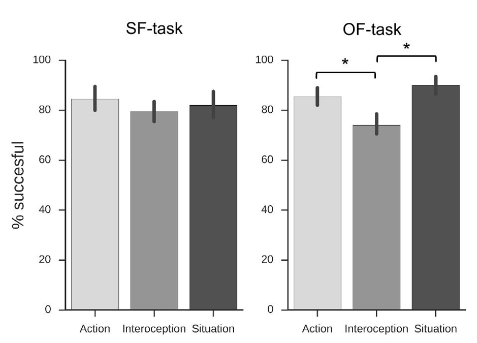
Figure A.1: Mean percentage of trials successfully executed for the SF-task (left panel) and OF-task (right panel). Error bars indicate 95% confidence intervals. A one-way ANOVA of the success-rates of the SF-task (left-panel) indicated no significant overall differences, F(2, 17) = 1.03, p = 0.38. In the OF-task (right panel) however, a one-way ANOVA indicated that success-rates differed significantly between classes, F(2, 17) = 17.74, p < 0.001. Follow-up pairwise comparisons (Bonferroni corrected, two tailed) revealed that interoception-trials (M = 74.00, SE = 2.10) were significantly less successful (p < 0.001) than both action-trials (M = 85.50, SE = 1.85) and situation trials (M = 90.00, SE = 1.92).
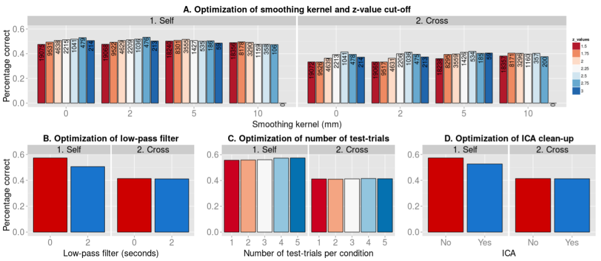
Figure A.2: Results of the parameter-optimization procedure. Reported scores reflect the classification scores averaged over subjects and classes (i.e. the diagonal of the confusion matrix). All optimization analyses were iterated 5000 times. A) Classification results for different smoothing kernels (0, 2, 5, and 10 mm) and z-value threshold for differentiation scores during feature selection (see MVPA pipeline section in the main text for a description of the particular feature selection method we employed). Numbers reflect the average number of voxels selected across iterations. B) Classification results of using a low-pass filter (2 seconds) or not. C) Classification results for different numbers of test-trials per class (1 to 5). D) Classification results when preprocessing the data with Independent Component Analysis (ICA) or not.
| Parameter | Options | Final choice |
|---|---|---|
| Smoothing kernel | 0 mm, 2 mm, 5 mm, 10 mm | 5 mm |
| Feature selection threshold | 1.5, 1.75, 2, 2.25, 2.5, 2.75, 3 | 2.3 |
| Number of test-trials | 1, 2, 3, 4, 5 | 4 |
| Low-pass filter | 2 seconds vs. none | None |
| ICA denoising | ICA vs. no ICA | No ICA |
| Note: The first set of parameters we evaluated in the optimization-set were different smoothing factors and feature selection thresholds (see MVPA pipeline section in the main text). On average, across the self- and cross-analysis, a 5 mm smoothing kernel yielded the best results in combination with a feature selection threshold of 2.25, which we rounded up to 2.3 as this number represents a normalized (z-transformed) score, which corresponds to the top 1% scores within a normal distribution. Next, the difference between using a low-pass (of 2 seconds, i.e. 1 TR) versus none was assessed, establishing no low-pass filter as the optimal choice. Next, different numbers of test-trials (1 to 5) per class per iteration were assessed. Four trials yielded the best results. Lastly, the effect of “cleaning” the data with an independent component analysis was examined (FSL: MELODIC and FIX; Salimi-Khorshidi et al., 2014). Not performing ICA yielded the best results. These parameters – 5 mm smoothing kernel, 2.3 feature selection thresholded, no low-pass filter, and four test-trials per iteration – were subsequently used in the analysis of the validation set. |
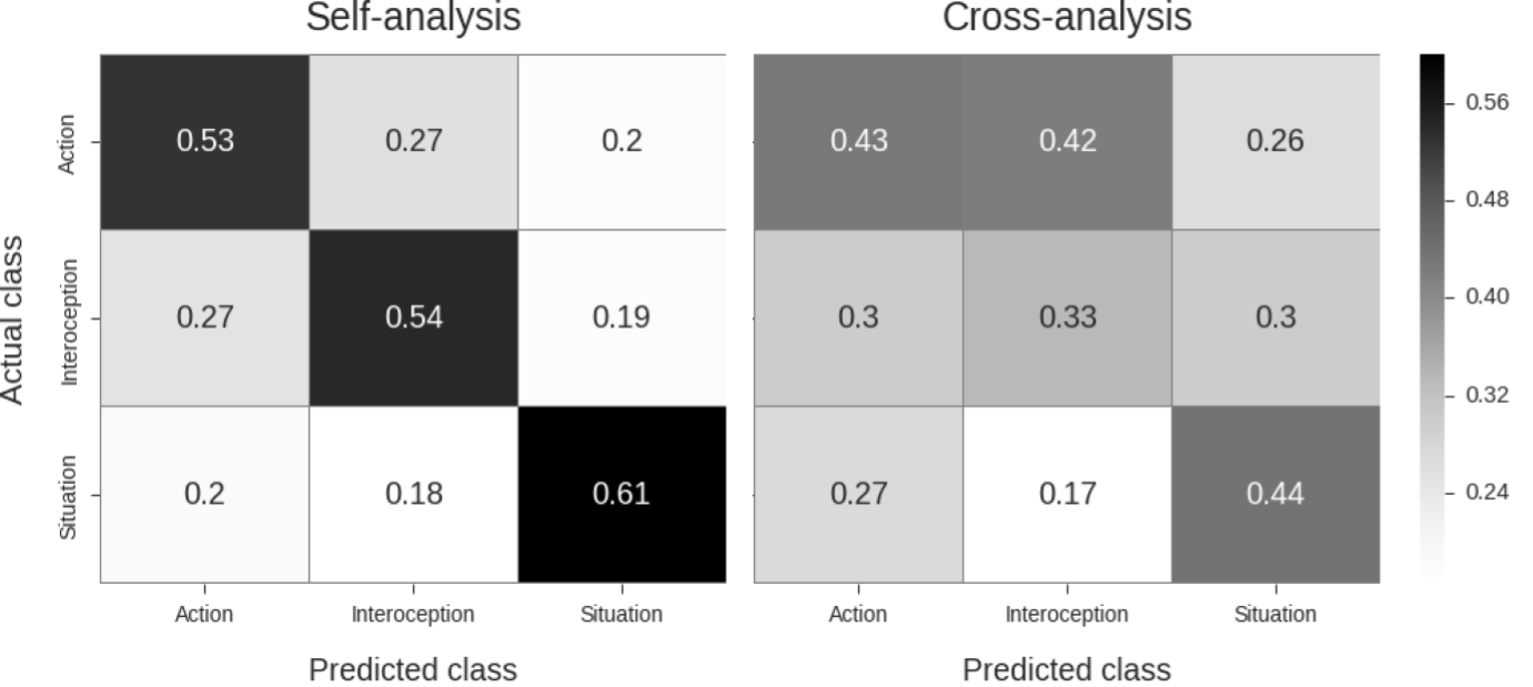
Figure A.3: Confusion matrices displaying precision-values yielded by the classification analysis of the optimization dataset with the final set of parameters. Because no permutation statistics were calculated for the optimization set, significance was calculated using a one-sample independent t-test against chance-level classification (i.e. 0.333) for each cell in the diagonal of the confusion matrices. Here, all t-statistics use a degrees of freedom of 12 (i.e. 13 subjects - 1) and are evaluated against a significance level of 0.05, Bonferroni-corrected. For the diagonal of the self-analysis confusion matrix, all values were significantly above chance-level, all p < 0.0001. For the diagonal of the cross-analysis confusion matrix, both the action (43% correct) and situation (44% correct) classes scored significantly above chance, p = 0.014 and p = 0.0007 respectively. Interoception was classified at chance level, p = 0.99, which stands in contrast with the results in the validation-set.
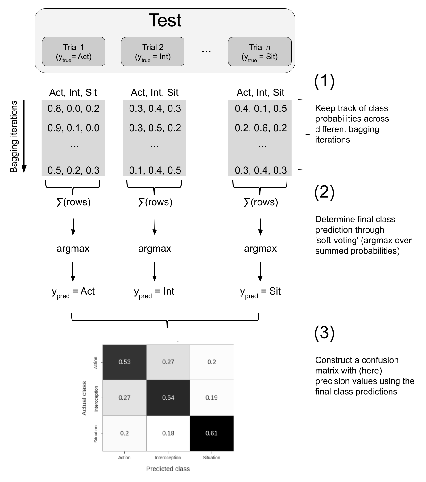
Figure A.4: Schematic overview of the bagging procedure. Class probabilities across different bagging iterations are summed and the class with the maximum probability determines each trial’s final predicted class, which are subsequently summarized in a confusion matrix on which final recall/precision scores are calculated.
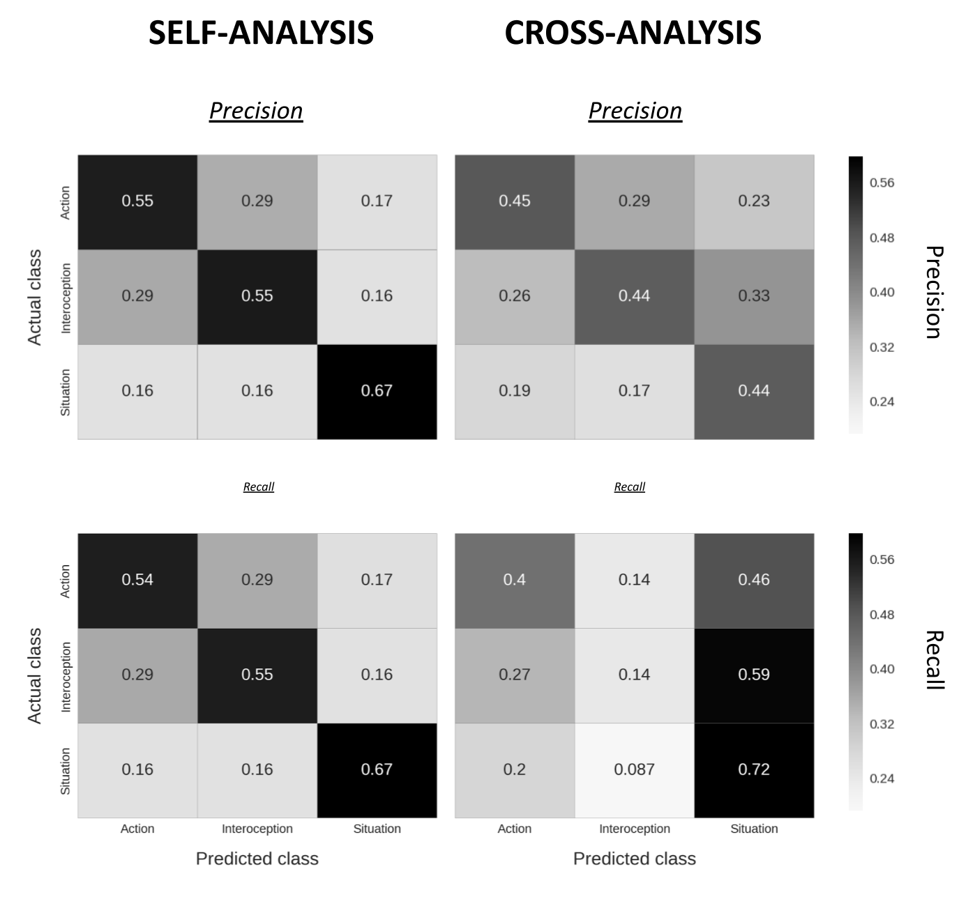
Figure A.5: (ref:caption-fig-shared-states-S5)
(ref:caption-fig-shared-states-S5) A comparison between precision and recall confusion matrices of the self- and cross-analysis of the validation dataset. Precision refers to the amount of true positive predictions of a given class relative to all predictions for that class. Recall refers to the amount of true positive predictions of a given class relative to the total number of samples in that class. In the self-analysis, all classes were decoded significantly above chance for both precision and recall (all p < 0.001). In the cross-analysis, all classes were decoded significantly above chance for precision (all p < 0.001); for recall both action and situation were decoded significantly above chance (p = 0.0013 and p < 0.001, respectively), while interoception was decoded below chance. All p-values were calculated using a permutation test with 1300 permutations (as described in the Methods section in the main text). When comparing precision and recall scores for both analyses, precision and recall showed very little differences in the self-analysis, while the cross-analysis shows a clear difference between metrics, especially for interoception and situation. For the interoception class, the relatively high precision score (44%) compared to its recall score (14%) suggests that trials are very infrequently classified as interoception, but when they are, it is (relatively) often correct. For the situation class, the relatively high recall score (72 %) compared to its precision score (44%) suggests that situation is strongly over-classified, which is especially clear in the lower-right confusion matrix, which indicates that 59% of the interoception-trials are misclassified as situation-trials.
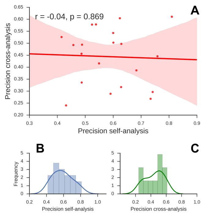
Figure A.6: Relation between self- and cross-analysis scores across subjects and their respective distributions. Note that the scores here represent the average of the class-specific precision scores. A) There is no significant correlation between precision-scores on the self-analysis and the corresponding scores on the cross-analysis, r = -0.04, p = .86, implying that classification scores in the self-analysis is not predictive of scores in the cross-analysis. B) The distribution of precision-scores in the self-analysis, appearing to be normally distributed. C) The distribution of precision-scores in the cross-analysis, on the other hand, appears to be bimodal, with one group of subjects having scores around chance level (0.333) while another group of subjects clearly scores above chance level (see individual scores and follow-up analyses in (ref:fig-shared-states-S4).
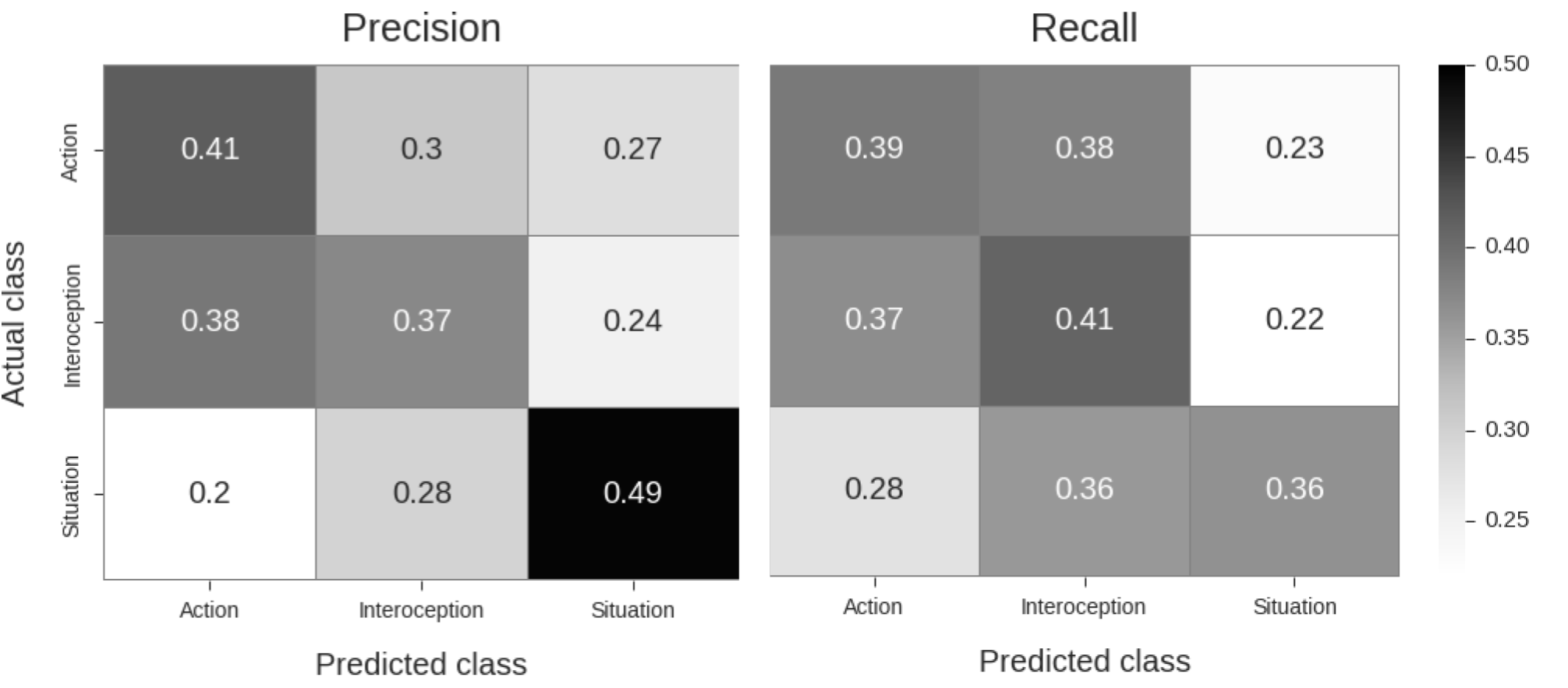
Figure A.7: Confusion matrices with precision (left matrix) and recall (right matrix) estimates of the other-to-self decoding analysis. The MVPA-pipeline used was exactly the same as for the (self-to-other) cross-analysis in the main text. P-values corresponding to the classification scores were calculated using a permutation analysis with 1000 permutations of the other-to-self analysis with randomly shuffled class-labels. Similar to the self-to-other analysis, the precision-scores for all classes in the other-to-self analysis were significant, p(action) < 0.001, p(interoception) = 0.008, p(situation) < 0.001. For recall, classification scores for action and interoception were significant (both p < 0.001), but not significant for situation (p = 0.062). The discrepancy between the self-to-other and other-to-self decoding analyses can be explained by two factors. First, the other-to-self classifier was trained on fewer samples (i.e. 90 trials) than the self-to-other classifier (which was trained on 120 trials), which may cause a substantial drop in power. Second, the preprocessing pipeline and MVPA hyperparameters were optimized based on the self-analysis and self-to-other cross-analysis. Given the vast differences between the nature of the self- and other-data, these optimal preprocessing and MVPA hyperparameters for the original analyses may not cross-validate well to the other-to-self decoding analysis.
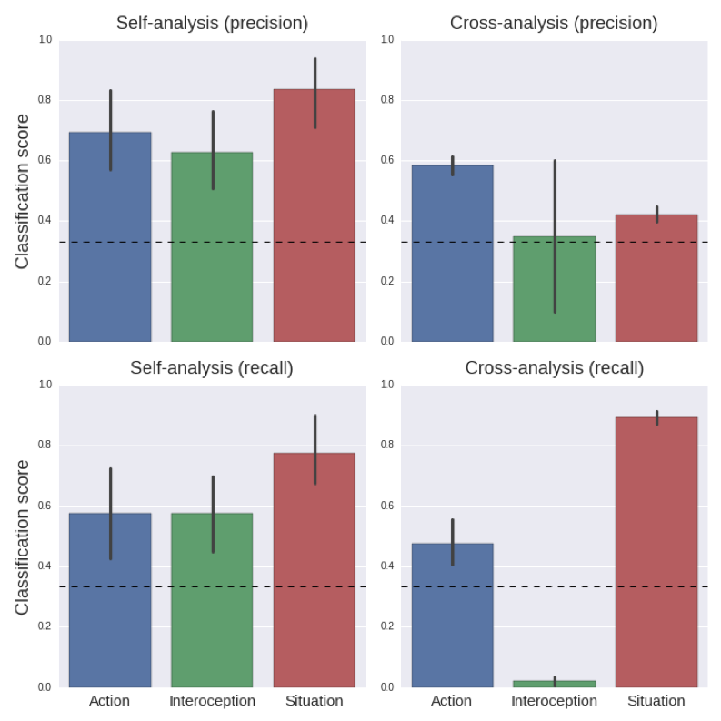
Figure A.8: Results of MVPA analyses using condition-average voxel patterns across subjects instead of single-trial patterns within subjects.
Here, patterns are estimated in a GLM in which each condition, as opposed to each trial, is modeled with a single regressor, from which whole-brain t-value patterns were extracted. In this condition-average multi-voxel pattern analysis, condition-average patterns across subjects were used as samples. The condition-average patterns were extracted from the univariate first-level contrasts. In total, this yielded 120 samples for the self-data (3 conditions x 2 runs x 20 participants) and 60 samples for the other-data (3 conditions * 20 participants). For these analyses, the same hyperparameters were used as the original analyses reported in the main text, except with regard to the cross-validation and bagging procedure. Here, we used (stratified) 10-fold cross-validation without bagging. The upper panels show precision scores (per class) for the self- and (self-to-other) cross-analysis; the lower panels show results from the same analyses but expressed in recall-estimates (error bars indicate 95% confidence intervals). Apart from interoception in the cross-analysis (both precision and recall), all scores were significant (p < 0.001) in a permutation test with 1000 permutations. These results largely replicate our findings as reported in the main text. This suggests that the neural patterns involved in self-focused emotional imagery and other-focused emotion understanding are relatively consistent in terms of spatial distribution across subjects. We explain this consistency by assuming that our tasks engage domain-general psychological processes that are present in all individuals.
| Subject nr. | Self-analysis precision | Cross-analysis precision | Session | Part of optimization-set? |
|---|---|---|---|---|
| 1 | 0.758 | 0.445 | 2 | y |
| 2 | 0.487 | 0.336 | 2 | y |
| 3 | 0.629 | 0.316 | 1 | y |
| 4 | 0.524 | 0.577 | 2 | y |
| 5 | 0.457 | 0.492 | 1 | y |
| 6 | 0.741 | 0.296 | 2 | y |
| 7 | 0.600 | 0.542 | 1 | y |
| 8 | 0.431 | 0.240 | 2 | y |
| 9 | 0.629 | 0.497 | 1 | y |
| 10 | 0.734 | 0.268 | 2 | y |
| 11 | 0.683 | 0.386 | 1 | y |
| 12 | 0.415 | 0.525 | 2 | y |
| 13 | 0.623 | 0.604 | 1 | y |
| 14 | 0.810 | 0.610 | 1 | n |
| 15 | 0.538 | 0.578 | 1 | n |
| 16 | 0.486 | 0.455 | 1 | n |
| 17 | 0.549 | 0.415 | 1 | n |
| 18 | 0.488 | 0.494 | 1 | n |
| 19 | 0.590 | 0.289 | 1 | n |
| 20 | 0.600 | 0.502 | 1 | n |
| Note: Supplementary Table 3 suggests individual variability in the extent to which neural resources are shared between self- and other-focused processes. In the SF-task all subjects demonstrated a mean classification score well above .33 (i.e., score associated with chance). When generalizing the SF-classifier to the OF-task, however, the classification scores appear to be bimodally distributed (see Supplementary Figure 5C). As can be seen in Table 3, some subjects demonstrated a relatively high mean classification score (i.e., > .45), whereas other subjects demonstrated a classification score at chance level or lower. Note that there is no significant difference between the OF classification scores for subjects who participated in the experiment for the first or second time (“Session” column in table; t(18) = 1.73, p = 0.10), nor for subjects who were or were not part of the optimization-set (“Part of optimization-set?” column in table; t(18) = -.95, p = 0.35), suggesting that inclusion in the optimization-set or session ordering is not a confound in the analyses. Regarding individual variability in self-other neural overlap, it is important to note that in the field of embodied cognition, there is increasing attention for the idea that simulation is both individually and contextually dynamic (Oosterwijk & Barrett, 2014; Winkielman, Niedenthal, Wielgosz & Kavanagh, 2015; see also Barrett, 2009). To better distinguish between meaningful individual variation and variation due to other factors (e.g., random noise), future research should test a priori formulated hypotheses about how and when individual variation is expected to occur. |
| Brain region | k | Max | Mean | Std |
|---|---|---|---|---|
| Frontal pole | 1827 | 5.05 | 2.35 | 0.52 |
| Occipital pole | 1714 | 5.15 | 2.45 | 0.56 |
| Supramarginal gyrus anterior | 1573 | 7.48 | 2.84 | 0.91 |
| Lateral occipital cortex superior | 1060 | 4.52 | 2.18 | 0.39 |
| Lateral occipital cortex inferior | 923 | 4.73 | 2.36 | 0.49 |
| Angular gyrus | 856 | 4.52 | 2.24 | 0.40 |
| Supramarginal gyrus posterior | 806 | 4.49 | 2.29 | 0.45 |
| Middle temporal gyrus temporo-occipital | 798 | 4.00 | 2.33 | 0.48 |
| Temporal pole | 711 | 4.38 | 2.37 | 0.54 |
| Precentral gyrus | 568 | 3.54 | 2.14 | 0.31 |
| Superior temporal gyrus posterior | 549 | 3.64 | 2.27 | 0.41 |
| Superior frontal gyrus | 510 | 3.83 | 2.18 | 0.38 |
| Postcentral gyrus | 489 | 4.61 | 2.43 | 0.60 |
| Inferior frontal gyrus parstriangularis | 488 | 4.22 | 2.35 | 0.50 |
| Inferior frontal gyrus parsopercularis | 441 | 3.54 | 2.14 | 0.31 |
| Middle temporal gyrus posterior | 417 | 5.68 | 2.34 | 0.52 |
| Occipital fusiform | 400 | 4.28 | 2.14 | 0.37 |
| Middle temporal gyrus anterior | 398 | 5.68 | 2.58 | 0.76 |
| Middle frontal gyrus | 300 | 3.01 | 2.06 | 0.25 |
| Precuneus | 282 | 3.34 | 2.14 | 0.31 |
| Note: Brain regions were extracted from the Harvard-Oxford (bilateral) Cortical atlas. A minimum threshold for the probabilistic masks of 20 was chosen to minimize overlap between adjacent masks while maximizing coverage of the entire brain. The column k represents the absolute number of above-threshold voxels in the masks. The columns Max, Mean, and Std represent the maximum, mean, and standard deviation from the t-values included in the masks. Note that the t-values, corresponding to the mean weight across subjects normalized by the standard error of the weights across subjects (after correcting for a positive bias when taking the absolute of the weights), were thresholded at a minimum of 1.75, referring to a p-value of 0.05 of a one-sided t-test against zero with 19 degrees of freedom (i.e. n – 1). Note that this t-value map was not corrected for multiple comparisons, and is intended to visualize which regions in the brain were generally involved in our sample of subjects. The X, Y, and Z columns represent the MNI152 (2mm) coordinates of the peak (i.e. max) t-value for each listed brain region. |