E Supplement to Chapter 6
E.1 Supplementary methods
Below, we describe the methodology behind hypothesis kernel analysis and noise ceiling estimation in more detail.
E.1.1 Hypothesis kernel analysis (in detail)
E.1.1.1 Step 1: encoding mappings
The first step in our method is the embedding of hypotheses in a common space. In the context of AU-emotion mappings, this amounts to formalizing these mappings as points in “AU space”. Here, AU space is a multidimensional space in which each of the AUs under consideration represents one dimension and each AU-emotion mapping (e.g., “disgust = AU9 + AU10”) can be represented as a single point in this space. For example, suppose that we only consider a limited set of five AUs (AU4, AU9, AU10, AU12, and AU23). We then can represent the hypothetical mapping “disgust = AU9 + AU10”, \(\mathbf{M}_{\mathrm{disgust}}\), as a point with five coordinates (i.e., a vector), which value indicates whether a given AU is part of the hypothesized configuration (1) or not (0):
\[\begin{equation} \mathbf{M}_{\mathrm{disgust}} = \begin{bmatrix} 0 & 1 & 1 & 0 & 0 & 0 \end{bmatrix} \end{equation}\]
Note that, in the above example, values at the positions of hypothesized AUs are all encoded as 1, which implies that each AU within the configuration is expressed equally intensely. This does not have to be the case; if, for example, the aforementioned mapping hypothesized that disgust is expressed with a combination of AU9 at 100% intensity but AU10 at 50% intensity, then its embedding can be expressed as follows:
\[\begin{equation} \mathbf{M}_{\mathrm{disgust}} = \begin{bmatrix} 0 & 1 & .5 & 0 & 0 & 0 \end{bmatrix} \end{equation}\]
For simplicity, we assume in this example that each hypothesized AU is expressed at equal intensity (such that vectors are binary). Importantly, many studies outline mappings with regard to multiple emotions, which we will refer to here as classes. For this example, we assume that our hypothetical mapping \(\mathbf{M}\) limits its mappings to the six basic emotions. Specifically, suppose that mapping \(\mathbf{M}\) outlines, in addition the the previously defined happiness mapping, specific hypothetical AU-emotion mappings for the following categorical emotions:
- anger = AU4 + AU5 + AU7
- disgust = AU9 + AU15
- fear = AU1 + AU2 + AU4 + AU7 + AU26
- sadness = AU1 + AU4 + AU15
- surprise = AU1 + AU2 + AU5 + AU26
Accordingly, we can encode the entire set of AU-emotion mappings for a given mapping, \(\mathbf{M}\), with \(C\) classes and \(D\) dimensions into a \(C \times D\) matrix, by vertically stacking the \(C\) different row mapping vectors. For our hypothetical mapping, \(\mathbf{M}\), its associated “mapping matrix” would look like the following:
\[\begin{equation} \mathbf{M} = \begin{bmatrix} 0 & 0 & 1 & 1 & 0 & 1 & 0 & 0 & 0 & 0 \\ 0 & 0 & 0 & 0 & 0 & 0 & 1 & 0 & 1 & 0 \\ 1 & 1 & 1 & 0 & 0 & 1 & 0 & 0 & 0 & 1 \\ 0 & 0 & 0 & 0 & 1 & 0 & 0 & 1 & 0 & 0 \\ 1 & 0 & 1 & 0 & 0 & 0 & 0 & 0 & 1 & 0 \\ 1 & 1 & 0 & 1 & 0 & 0 & 0 & 0 & 0 & 1 \end{bmatrix} \end{equation}\]
where its rows represent the different classes (categorical emotions) and the columns the involvement of a specific AU. Note that although the above represents a hypothetical mapping, its sparsity is something we would expect, as facial expressions are unlikely to be generated by a full (dense) set of action units (Yu et al., 2012).
E.1.1.2 Step 2: encoding stimuli
In the previous section we outlined how to formalize AU-emotion mappings as points (or, equivalently, vectors) in AU space. One way to evaluate these formalized mappings is to subject them to actual categorical emotion ratings from human participants in response to stimuli with known AU configurations. Ideally, the stimuli from such an experiment sample the AU space as densely and uniformly as possible in order not to bias the results towards hypothesized mappings. Many experiments on facial emotion expressions, however, use posed and stereotyped stimuli (e.g., facial expressions of intense joy or anger), which cover only a small part of the entire AU space and thus do not allow for unbiased evaluation of AU-based theories. In contrast, reverse correlation-based experiments, which are characterized by randomly and parametrically varying the input space (defined by AU configurations) and collection of resulting percepts (here: perception of categorical emotion) do not impose such constraints (Jack et al., 2017) and thus present an ideal type of dataset to subject to our formalized AU-emotion mappings.
In reference to our previously defined hypothetical 10-dimensional AU space, assume that we have categorical emotion ratings \(e\) from a set of emotions \(E\) (\(e \in E\)) in response to a collection of \(N\) facial expression stimuli parameterized with random AU configurations, drawn from the same 10-dimensional AU space discussed before. With such data, we can encode the stimuli in AU space in the same way we did in the previous section for AU-emotion mappings, i.e., we can quantify each stimulus, \(\mathbf{S}_{i}\), as a 10-dimensional “stimulus vector” containing nonzero values at positions associated with active AUs for that stimulus and zeros elsewhere. Note that, as is the case with mapping vectors, the stimulus vector’s nonzero values at positions associated with active AUs can be all ones (if assumed to be equally “active”) or be values proportional to the amplitude (or “activity”) of the active AUs.
For example, suppose that stimulus \(\mathbf{S}_{i}\) contains AU1, AU5, and AU26 with amplitudes 0.1, 0.5, and 0.8 respectively (where an amplitude of 1 would represent an AU at maximum intensity). Then, formally, we can represent this particular stimulus, \(\mathbf{S}_{i}\), as the following stimulus vector:
\[\begin{equation} \mathbf{S}_{i} = \begin{bmatrix} .1 & 0 & 0 & .5 & 0 & 0 & 0 & 0 & 0 & .8 \end{bmatrix} \end{equation}\]
In case of multiple stimuli (\(\mathbf{S}_{i}\) for \(i = \{1, \dots, N\}\)), their mapping vectors can be vertically stacked in a single \(N \times D\) “stimulus matrix”, \(\mathbf{S}\).
Given that both a mapping (\(\mathbf{M}\)) and set of stimuli (\(\mathbf{S}\)) are encoded as matrices in the same \(D\)-dimensional AU space, we can discuss using kernels to generate quantitative predictors for stimuli given a particular theory.
E.1.1.3 Step 3: kernel functions
Kernel functions (or simply kernels) are functions that are, broadly speaking, measures of similarity between two vectors. Applied to our use case, we use kernel functions (\(\kappa\)) to quantify the similarity, i.e. “closeness” in AU space, (\(\phi\)) between a stimulus with a known AU configuration (\(\mathbf{S}_{i}\)) and a mapping vector for a specific emotion, indexed by \(j\) (\(\mathbf{M}_{j}\), e.g., happiness)21:
\[\begin{equation} \phi_{ij} = \kappa(\mathbf{S}_{i}, \mathbf{M}_{j}) \end{equation}\]
Most (linear) kernel functions are based on the dot (inner) product between the two vectors. In the current study, we primarily use the cosine kernel, which normalizes the dot product between two vectors with the product of their L2 (Euclidean) norm:
\[\begin{equation} \kappa(\mathbf{S}_{i}, \mathbf{M}_{j}) = \frac{\mathbf{S}_{i}\mathbf{M}_{j}^{T}}{\left\Vert \mathbf{S}_{i} \right\Vert \left\Vert \mathbf{M}_{j} \right\Vert} \end{equation}\]
Without such normalization, similarity values monotonically increase with increasing magnitudes of the stimulus vector, even if the stimulus vector increasingly deviates from the mapping.
E.1.1.4 Step 4: computing predictions
Although the similarity to a particular mapping vector can, generally speaking, be interpreted as being proportional to the evidence for that particular class, it is not strictly speaking a prediction. To generate a quantitative prediction for stimulus \(\mathbf{S}_{i}\) (i.e., \(\hat{e}_{i}\)), one needs to formulate a decision function that maps the data to a prediction. One possibility is to determine the prediction to be the emotion (across \(C\) classes) that maximizes its similarity, for some kernel function (\(\kappa\)), to the stimulus:
\[\begin{equation} \hat{e}_{i} = \underset{j}{\operatorname{\mathrm{argmax}}}\ \kappa(\mathbf{S}_{i}, \mathbf{M}_{j}) \end{equation}\]
In a slightly more sophisticated version of this decision function, we can generate probabilistic predictions instead of discrete predictions. To do so, we normalize the similarity vector using the softmax function, which returns a vector that sums to 1 such that their elements can be interpreted as probabilities (i.e., the probability of an emotion given a stimulus and mapping matrix):
\[\begin{equation} P(E_{j} | \mathbf{M}, \mathbf{S}_{i}) = \frac{\exp(\beta\phi_{ij})}{\sum_{j=1}^{C}\exp(\beta\phi_{ij})} \end{equation}\]
where \(\beta\) is the “inverse temperature” parameter — a scaling parameter — which distributes relatively more mass onto the largest values within the sequence of similarities. In our framework, we can treat this parameter as a model hyperparameter (i.e., a parameter that is not fit, but could be manually tuned using cross-validation). In our analyses, we use an inverse temperature parameter of 1 (see Supplementary Figure E.2 for a comparison of the effect of different parameter values on model performance).
E.1.1.5 Step 5: quantifying model performance
To evaluate the performance of each mapping, we can compare their (discrete or probabilistic) emotion predictions for a set of stimuli with emotion labels from participants who rated the same stimuli. In other words, we can quantitatively assess how well the theoretical predictions match with actual behavior. Model performance, or “score”, can be quantified using any function (\(q\)), or “metric”, that takes as inputs a set of predicted labels (\(\hat{e}\)) and a set of “true” labels (\(e\)) and returns a single number that summarizes the model performance, or “score”:
\[\begin{equation} \mathrm{score} = q(e, \hat{e}) \end{equation}\]
Instead of returning a single, class-average model performance estimate, some metrics are also able to return class-specific model performance scores. In our analyses, we used the “area under the curve of the receiver operating characteristic” (AUROC) which summarizes the quality of probabilistic predictions in a range from 0 to 1, where 0.5 is chance level performance and 1 is a perfect prediction. Note that our proposed method does not require a specific performance metric. We prefer to use AUROC as it can be used for both discrete and probabilistic predictions, is insensitive to class imbalance (i.e., unequal frequencies of target classes), and allows for class-specific performance estimates.
E.1.2 Noise ceiling estimation (in detail)
Suppose that, for a given dataset, we find that a particular mapping yields a (class-average) AUROC score of 0.8 — what can and should be concluded from this score? It is certainly above chance level (a score of 0.5) but also substantially below perfect performance (i.e., a score of 1). Here, we argue that one should not interpret performance relative to a theoretical maximum score, but relative to a noise ceiling & a concept borrowed from systems neuroscience (Lage-Castellanos et al., 2019) — which represents an upper bound that incorporates the within- and between-subject “variance” in ratings. In other words, a noise ceiling is a way to estimate an upper bound for predictive models that is adjusted for the “consistency” of the target variable.
One important reason to quantify a model’s noise ceiling is that is partitions the unexplained variance (i.e., part of the data that was not predicted correctly) into unexplained but in principle explainable variance (i.e., the noise ceiling minus the model performance) and “irreducible” noise (i.e., the theoretical maximum performance minus the noise ceiling; see Figure 6.3). The amount of explainable variance in turn quantifies how much there is to gain in terms of model improvement: if this component is large, one might consider different or more complex models; if this component is small (i.e., the model performance is at or near the noise ceiling), one can conclude that the model cannot be improved any further (which does not mean that it is the correct model, however). When applied in the context of AU-emotion mappings, the noise ceiling illustrates what portion of the variance in emotion inferences can be, in principle, explained by AUs.
While noise ceilings are routinely used in systems and cognitive neuroscience (Hsu et al., 2004; Huth et al., 2012; Kay et al., 2013; Nili et al., 2014), existing methods for estimating noise ceilings are limited to regression models (assuming a continuous target variable, usually some type of brain measurement). In the current study, however, we are dealing with classification models, as we are trying to predict a categorical target variable (i.e., categorical emotion ratings). Here, we propose a novel approach to estimate a noise ceiling for predictive performance of classification models.
A crucial and necessary element for most noise ceiling estimation methods, including the one proposed here, is the availability of repeated trials. Using repeated trials, the variance (or, inversely, the “consistency”) in the target variable can be estimated and used to estimate an upper bound on predictive performance. In other words, a noise ceiling formalizes the idea that a model can only perform as well as the consistency of subjects. Importantly, trials are considered to be “repeats” if their representation in the model is the same. Thus, if a model only considers AUs, then stimuli with the same AU configuration are considered repeats, even if they differ in other features (such as face identity). Moreover, repeated trials may occur “within subjects” (e.g., a trial with a particular AU configuration presented multiple times) or “between subjects” (e.g., a trial with a particular AU configuration presented to different subjects). Within-subject repeats can be used to estimate a within-subject noise ceiling when working with subject-specific models (which is common in cognitive neuroscience; Lage-Castellanos et al., 2019) between-subject repeats can similarly be used to estimate a between-subject noise ceiling when working with a single, between-subject model. While both within- and between-subject variance are expected to affect the noise ceiling, in this study we only consider between-subject variance (as our dataset only contains between-subject repeats).
To illustrate the computation of the noise ceiling (for a between-subject model), let us consider the following minimal example. Suppose three subjects rated the same two facial expression stimuli (\(\mathbf{S}_{1}\) and \(\mathbf{S}_{2}\)). As summarized in Table E.1, the ratings are inconsistent across subjects, i.e., not each stimulus is consistently rated as displaying the same emotion.
| Stimulus | Ratings subject 1 | Ratings subject 2 | Ratings subject 3 | Optimal pred. |
|---|---|---|---|---|
| \(\mathbf{S}_{1}\) | Anger | Disgust | Anger | Anger |
| \(\mathbf{S}_{2}\) | Disgust | Disgust | Anger | Disgust |
As mentioned, the noise ceiling represents an upper bound of predictive performance for a given set of observations. In other words, the noise ceiling (\(\mathrm{nc}\)) represents the performance that an optimal model would obtain:
\[\begin{equation} \mathrm{nc} = q(e, e_{\mathrm{optimal}}) \end{equation}\]
Here, the optimal model can be any conceivable type of model, but is constrained in one crucial aspect: it should make the same predictions for repeated observations. The reason for this constraint is that, to a model, repeated observations represent identical input (i.e., stimuli parameterized by their stimulus vector) and should logically receive the same prediction.
When working with discrete predictions (i.e., a single predicted label per trial), the optimal model predicts the mode across repeated observations. In our example scenario, the optimal model would thus predict \(\mathbf{S}_{1}\) as “Anger” and \(\mathbf{S}_{2}\) as “Disgust”. The noise ceiling is subsequently computed as the performance, for a particular performance metric (such as AUROC or simple accuracy), of this optimal model given the true labels. In our example above, the optimal model predicts two out of three ratings per stimulus correctly, resulting in a class-average AUROC noise ceiling of 0.6667.
The disadvantage of using discrete predictions when computing the noise ceiling is that it may result in multiple modes (e.g., a given stimulus might be rated “anger” in 50% of subjects and “disgust” in the other 50% of subjects). One could pick a random mode as the optimal prediction, but this may arbitrarily impact the class-specific noise ceiling for the classes represented by the tied modes. As an alternative, we suggest using probabilistic instead of discrete predictions. When working with probabilistic predictions, the optimal model does not predict the mode, but a probability distribution across labels equal to the proportion of each label. Formally, for a given stimulus, \(\mathbf{S}_{i}\), with \(R\) repeats, the probability of each class, \(P(E_{j})\), is computed as the proportion of labels, \(e_{i}\), equal to that class:
\[\begin{align} P(E_{j} | \mathbf{S}_{i}) = \frac{1}{R}\sum_{k=1}^{R} \boldsymbol{1}(e_{ik} = E_{j}) \end{align}\]
where \(\boldsymbol{1}\) represents an indicator function returning 1 when the emotion label \(e_{ik}\) is equal to emotion label \(E_{j}\) and 0 otherwise. Therefore, in our example data, the optimal prediction for each repetition of \(\mathbf{S}_{1}\) is [0.667, 0.333] and the optimal prediction for each repetition of \(\mathbf{S}_{2}\) is \([0.667, 0.333]\), where the numbers represent the probability of “Anger” and “Disgust” respectively. Similar to the noise ceiling based on discrete predictions, we can compute the noise ceiling as the performance, for a particular metric, of the optimal model given the true labels. In the above example, the class-average AUROC noise ceiling would coincidentally, just like in the scenario with discrete predictions, be 0.6667.
E.2 Supplementary figures
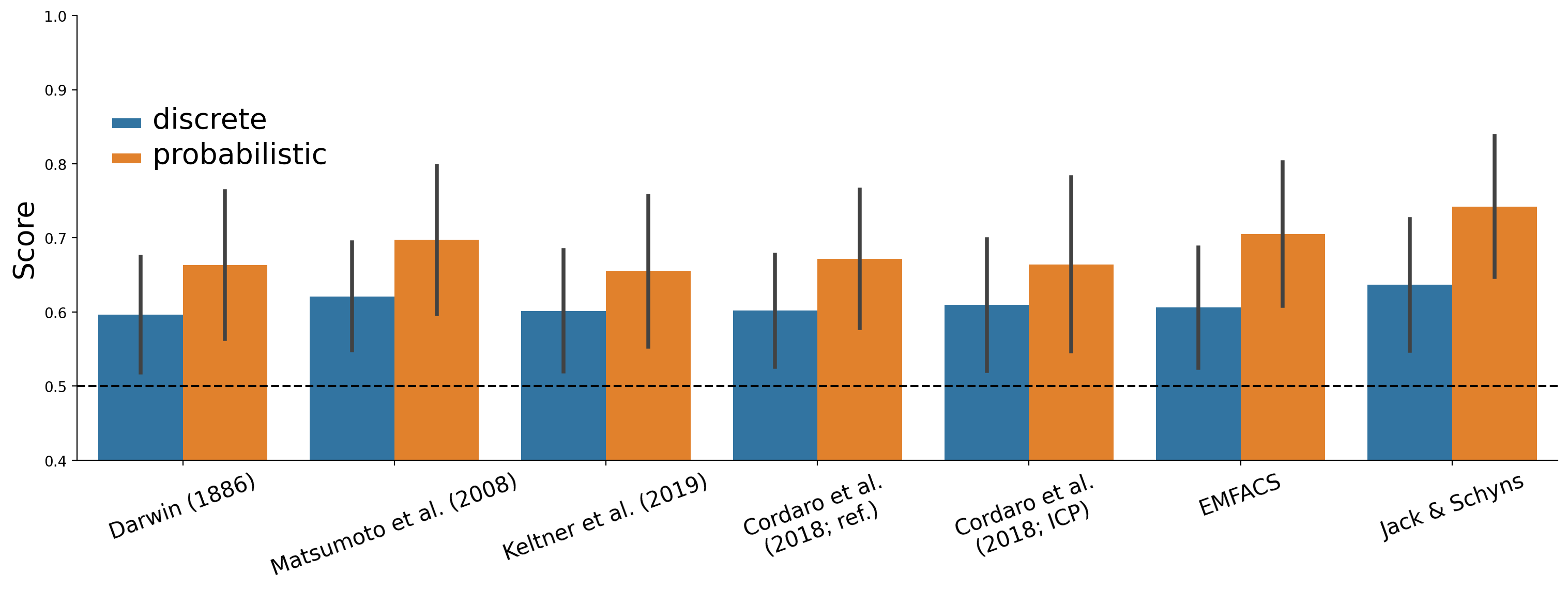
Figure E.1: Difference in class-average model performance (AUROC) between discrete and probabilistic predictions.
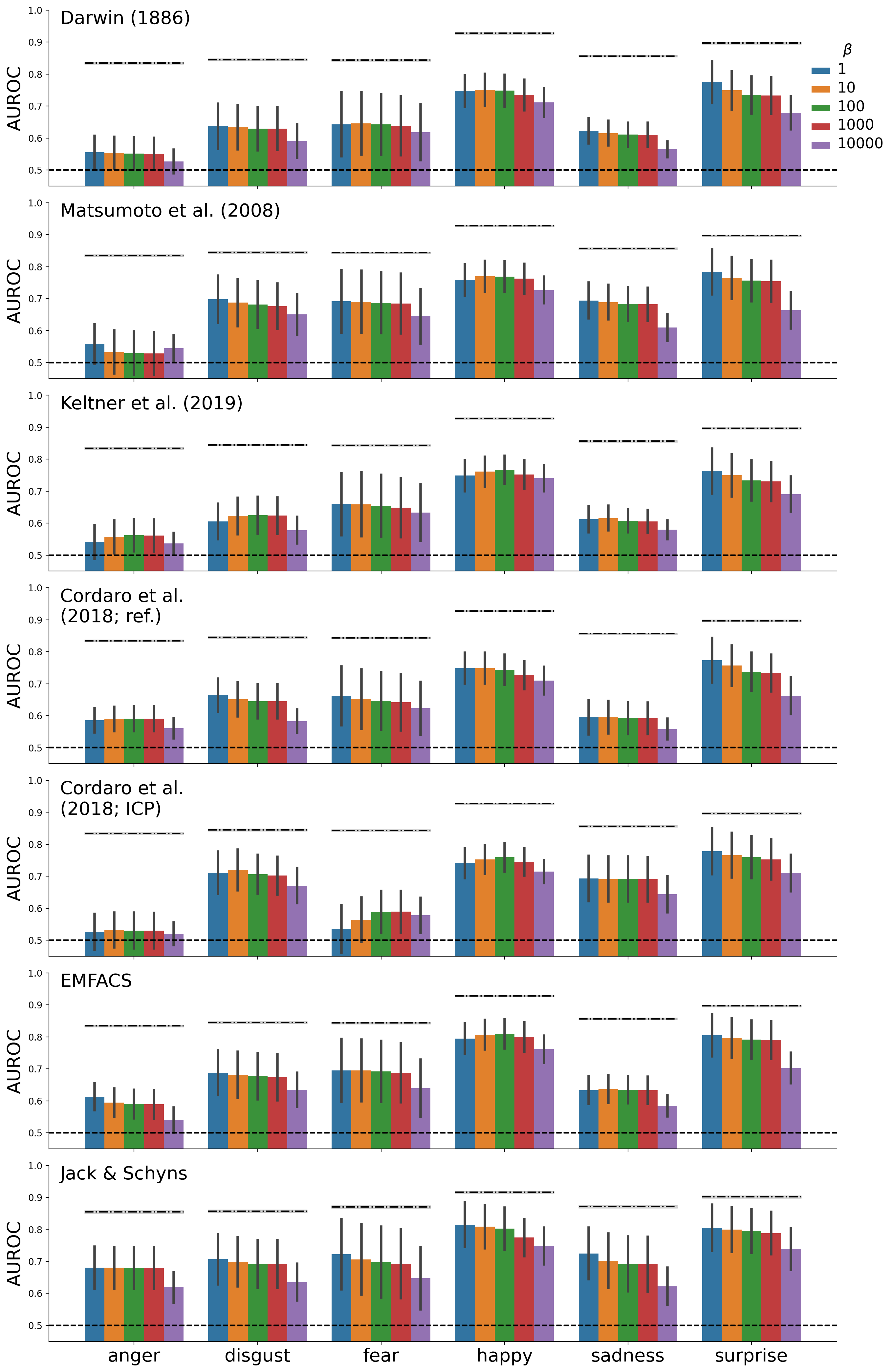
Figure E.2: Performance of different models for different values of the “inverse temperature” (\(\beta\)) parameter. A cosine kernel was used.
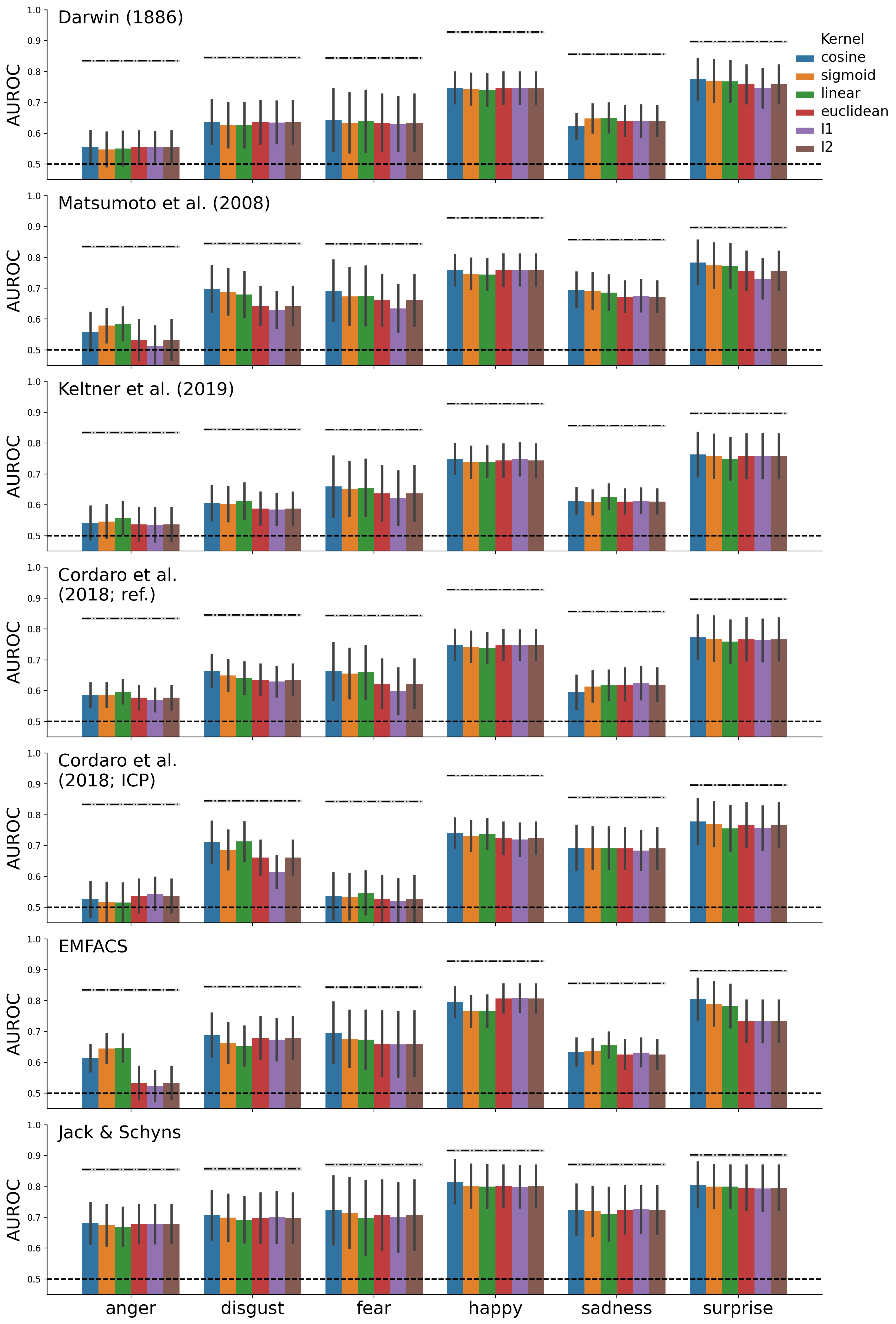
Figure E.3: Performance of different models for different kernel functions. The cosine, sigmoid, and linear kernels are measures of similarity, but the Euclidean, L1, and L2 kernels measure distance. For these distance functions, the distances were converted to similarities by inverting them. A fixed “inverse temperature” (\(\beta\)) parameter of 1 was used.
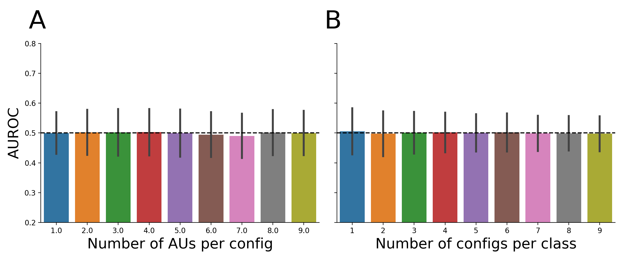
Figure E.4: Results from the simulation analysis with random mapping matrices in which the number of AUs per configuration (A) and the number of configurations per output class (B) were systematically varied. Bars represents the average AUROC score across 1000 simulations (error bars represent ±1 SD).
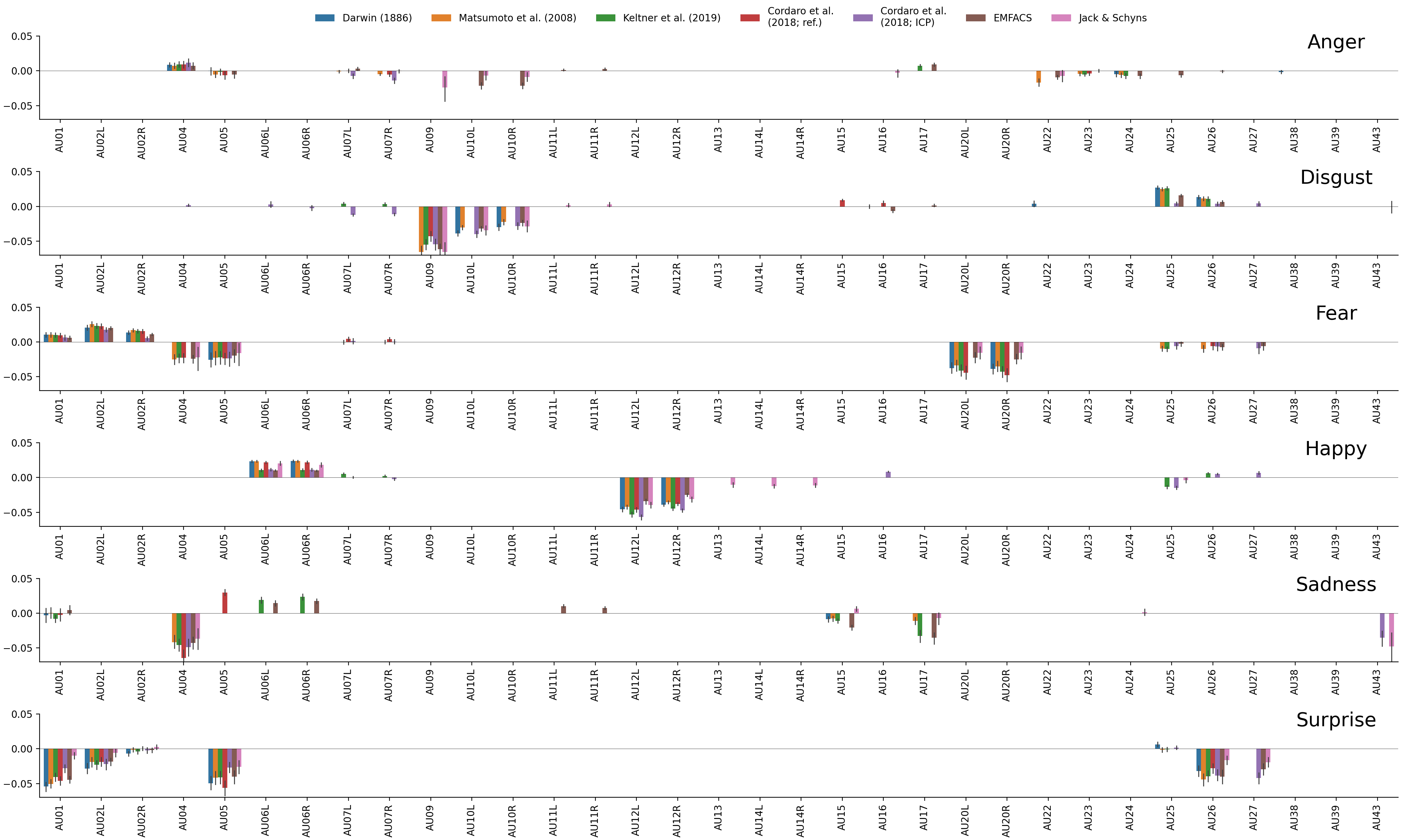
Figure E.5: Changes in model performance (AUROC) for each emotion and mapping after ablating an AU. Error bars indicate a 95% confidence interval obtained with 1000 bootstraps of the data.
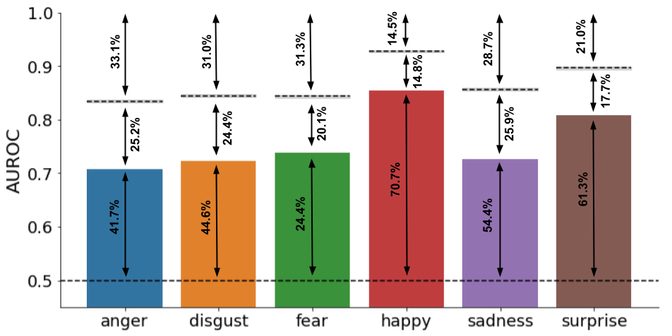
Figure E.6: . The proportion of explained AUROC (from 0.5 to top of bar), unexplained AUROC (from top of bar to noise ceiling), and irreducible noise/variance due to individual differences (from noise ceiling to 1.0) expressed as a percentage of the total AUROC.
| Emotion | AU | \(\Delta\) AUROC | Affected mappings |
|---|---|---|---|
| Anger | AU09 | -0.024 | Jack/Schyns |
| AU10R | -0.017 | EMFACS, Jack/Schyns | |
| AU10L | -0.017 | EMFACS, Jack/Schyns | |
| AU22 | -0.012 | Matsumoto, EMFACS, Jack/Schyns | |
| Disgust | AU09 | -0.057 | Matsumoto, Keltner, Cordaro (ref.), Cordaro (ICP), EMFACS, Jack/Schyns |
| AU10L | -0.035 | Darwin, Matsumoto, Cordaro (ICP), EMFACS, Jack/Schyns | |
| AU10R | -0.026 | Darwin, Matsumoto, Cordaro (ICP), EMFACS, Jack/Schyns | |
| AU25 | 0.020 | Darwin, Matsumoto, Keltner, Cordaro (ICP), EMFACS | |
| Fear | AU20R | -0.036 | Darwin, Matsumoto, Keltner, Cordaro (ref.), EMFACS, Jack/Schyns |
| AU20L | -0.034 | Darwin, Matsumoto, Keltner, Cordaro (ref.), EMFACS, Jack/Schyns | |
| AU04 | -0.024 | Matsumoto, Keltner, Cordaro (ref.), EMFACS, Jack/Schyns | |
| AU05 | -0.022 | All | |
| AU02L | 0.022 | Darwin, Matsumoto, Keltner, Cordaro (ref.), Cordaro (ICP), EMFACS | |
| AU02R | 0.013 | Darwin, Matsumoto, Keltner, Cordaro (ref.), Cordaro (ICP), EMFACS | |
| Happy | AU12L | -0.046 | All |
| AU12R | -0.038 | All | |
| AU14L | -0.012 | Jack/Schyns | |
| AU25 | -0.012 | Keltner, Cordaro (ICP), Jack/Schyns | |
| AU14R | -0.011 | Jack/Schyns | |
| AU13 | -0.010 | Jack/Schyns | |
| AU06R | 0.017 | All | |
| AU06L | 0.017 | All | |
| Sadness | AU04 | -0.048 | Matsumoto, Keltner, Cordaro (ref.), Cordaro (ICP), EMFACS, Jack/Schyns |
| AU43 | -0.040 | Cordaro (ICP), Jack/Schyns | |
| AU17 | -0.024 | Matsumoto, Keltner, EMFACS, Jack/Schyns | |
| AU15 | -0.010 | Darwin, Matsumoto, Keltner, EMFACS, Jack/Schyns | |
| AU05 | 0.030 | Cordaro (ref.) | |
| AU06R | 0.021 | Keltner, EMFACS | |
| AU06L | 0.017 | Keltner, EMFACS | |
| AU11L | 0.010 | EMFACS | |
| Surprise | AU01 | -0.041 | All |
| AU05 | -0.041 | All | |
| AU26 | -0.036 | All | |
| AU27 | -0.033 | Cordaro (ICP), EMFACS, Jack/Schyns | |
| AU02L | -0.021 | All | |
| Note: Only AUs with an absolute change in AUROC larger than 0.01 are included. The affected mappings column indicates which mappings contained this AU. |
Instead of using measures of similarity between two vectors (i.e., “kernels”), one could use measures of distances (\(\delta_{ij}\)) between two vectors instead and subsequently invert it to get a similarity score again, i.e., \(\phi_{ij} = \delta_{ij}^{-1}\). In practice, we find that it does not make much of a difference in terms of predictive performance (see Supplementary Figure E.3).↩︎