F Supplement to Chapter 7
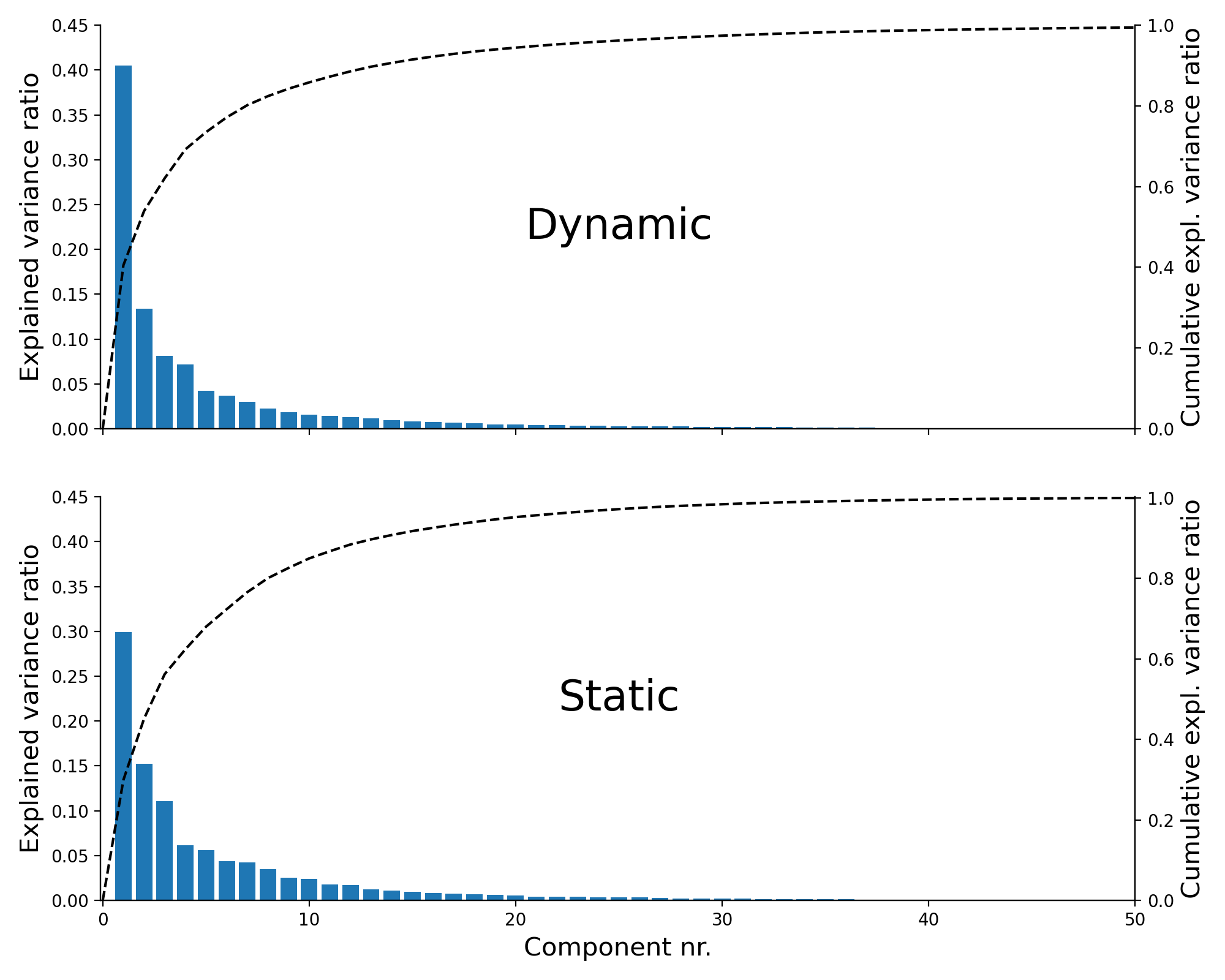
Figure F.1: The explained variance ratio of each PCA component (bars; left y-axis) and the cumulative explained variance ratio (dashed line; right y-axis) for the PCA done on the dynamic features (top) and static features (bottom).
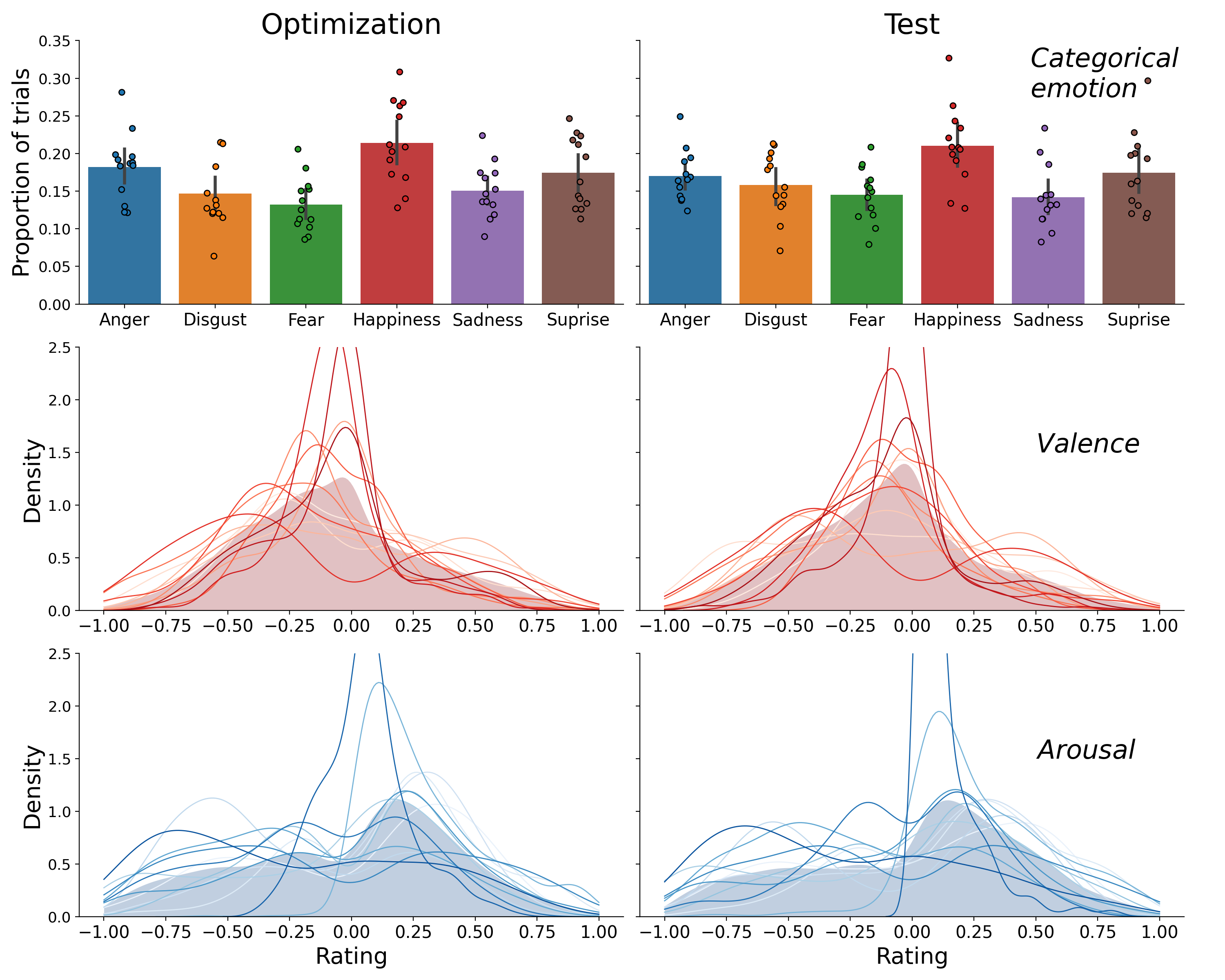
Figure F.2: Distribution of the categorical emotion labels (bars height represents the average proportion; dots represent individual participants; top) and the distribution of the valence ratings (middle) and arousal rating (bottom), shown separately for the optimization set (left) and test set (right). In the valence and arousal subplots, the filled area represents the distribution of the ratings pooled over participants and the lines represents the distribution of the ratings of individual participants. The valence and arousal distributions were created using kernel density estimation as implemented in the Python package seaborn (which uses the scipy function gaussian_kde with Scott’s rule for bandwidth selection).
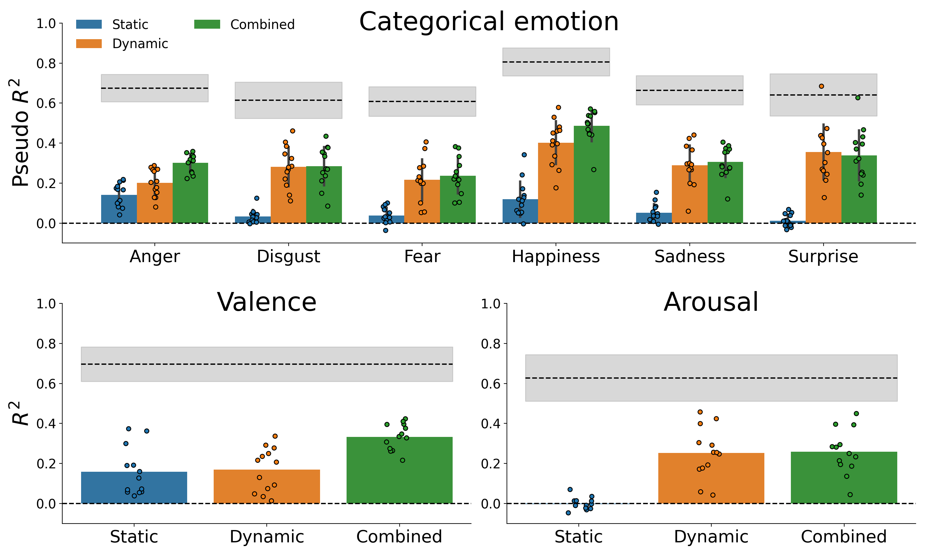
Figure F.3: Cross-validated model performance on optimization set, obtained by repeated 10-fold cross-validation. Because the optimization set does not contain repeated observations, the noise ceiling from the test set is visualized.
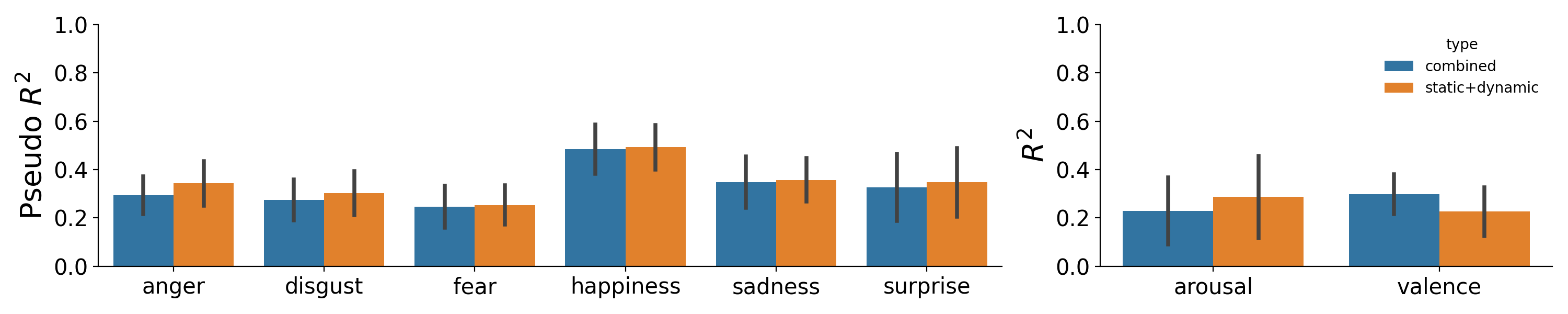
Figure F.4: Visualization of the comparison between the sum of static and dynamic model performance (orange) and the combined model performance (blue) for the categorical emotion model (left) and valence/arousal model (right).
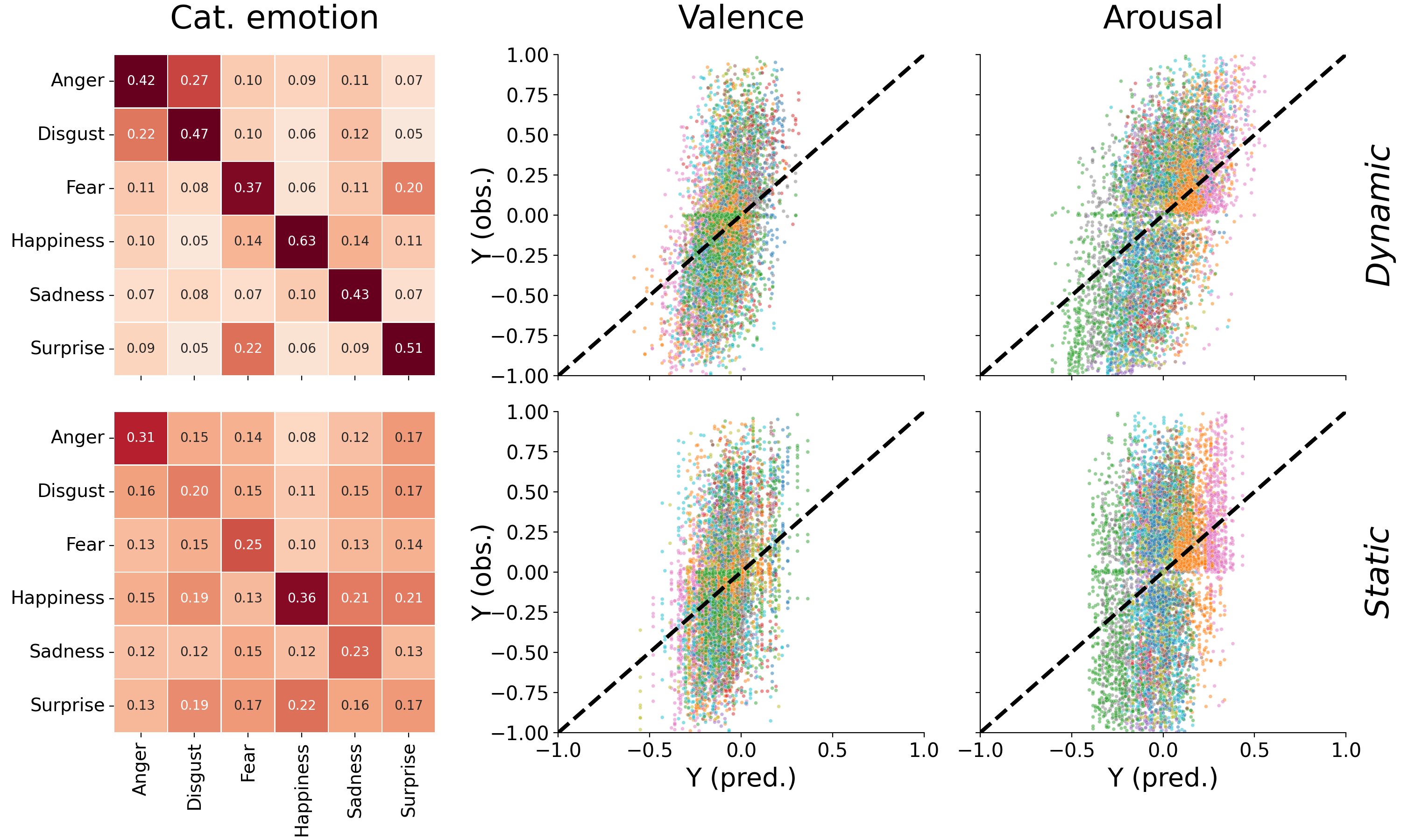
Figure F.5: Confusion matrices for the categorical emotions models (left) and regression plots for the valence model (middle) and arousal model (right), separately for the models based on dynamic information (top) and static information (bottom). The confusion matrices are normalized by the sum across rows, thus representing the recall (or sensitivity) on the diagonal. The categorical emotion classifier based on dynamic information relatively frequently misclassifies “anger” and “disgust” (and vice versa) as well as “surprise” and “fear” (and vice versa), replicating earlier findings from human ratings (Jack et al., 2014, 2009). In contrast, the confusion rates for the static emotion classifier are relatively uniform across categorical emotion pairs. Different colors in the regression plot represent ratings from different participants. The regression plots for the valence and arousal models (middle and right) show that both the models based on dynamic and static features tend to underestimate the magnitude of the predictions (i.e., few predictions are made above 0.5 or below -0.5). These attenuated predictions is a direct consequence of the strong regularization applied to the regression models (i.e., \(\lambda = 500\)), which causes the parameters (i.e., \(\hat{\beta}\)) to be shrunk towards zero, thus shrinking predictions (\(X\hat{\beta}\)) towards the mean as well.
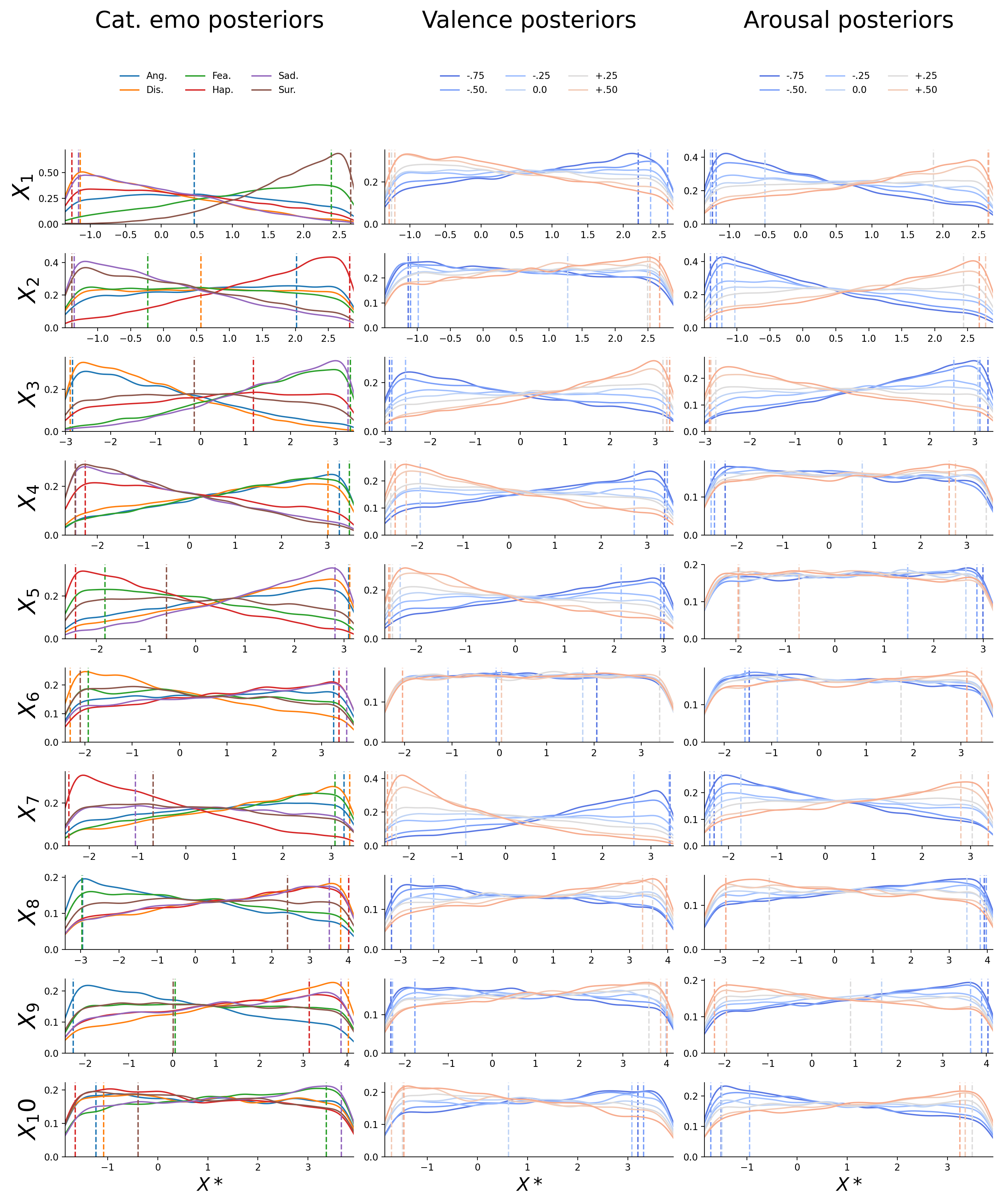
Figure F.6: Posterior distributions for the first ten dynamic features (\(X_{1}-X_{10}\); in rows) for the inverted categorical emotion model (left; different emotions as separate lines), the inverted valence model (middle; different levels as separate lines), and the inverted arousal model (right; different levels as separate lines). The dashed vertical lines represent the value chosen for the reconstructions (i.e., the midpoint of the 5% HDI interval). The drop at the edges of the posterior is an artifact induced by the kernel density estimation.
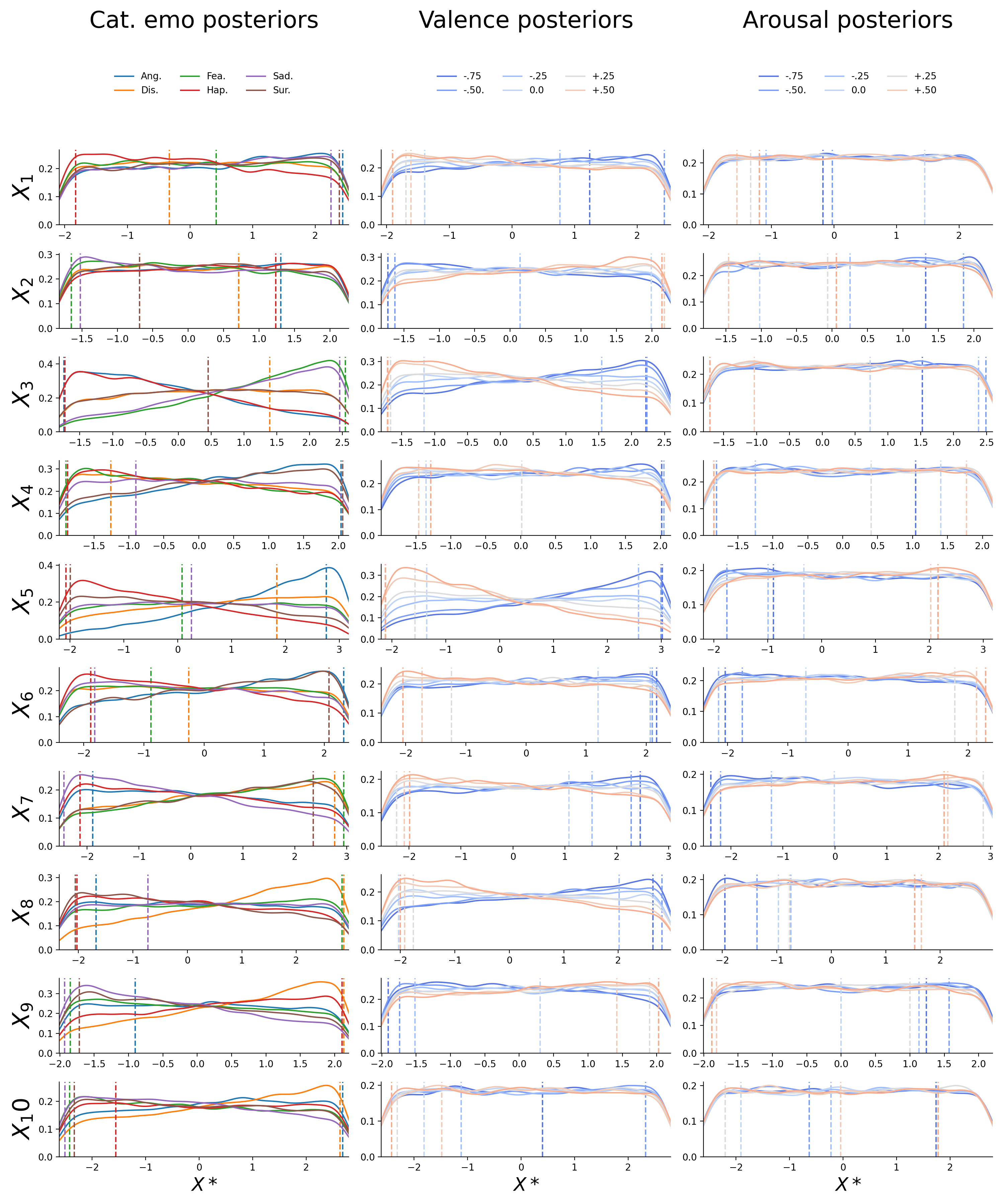
Figure F.7: Posterior distributions for the first ten static features (\(X_{1}-X_{10}\); in rows) for the inverted categorical emotion model (left; different emotions as separate lines), the inverted valence model (middle; different levels as separate lines), and the inverted arousal model (right; different levels as separate lines). The dashed vertical lines represent the value chosen for the reconstructions (i.e., the midpoint of the 5% HDI interval). The drop at the edges of the posterior is an artifact induced by the kernel density estimation.
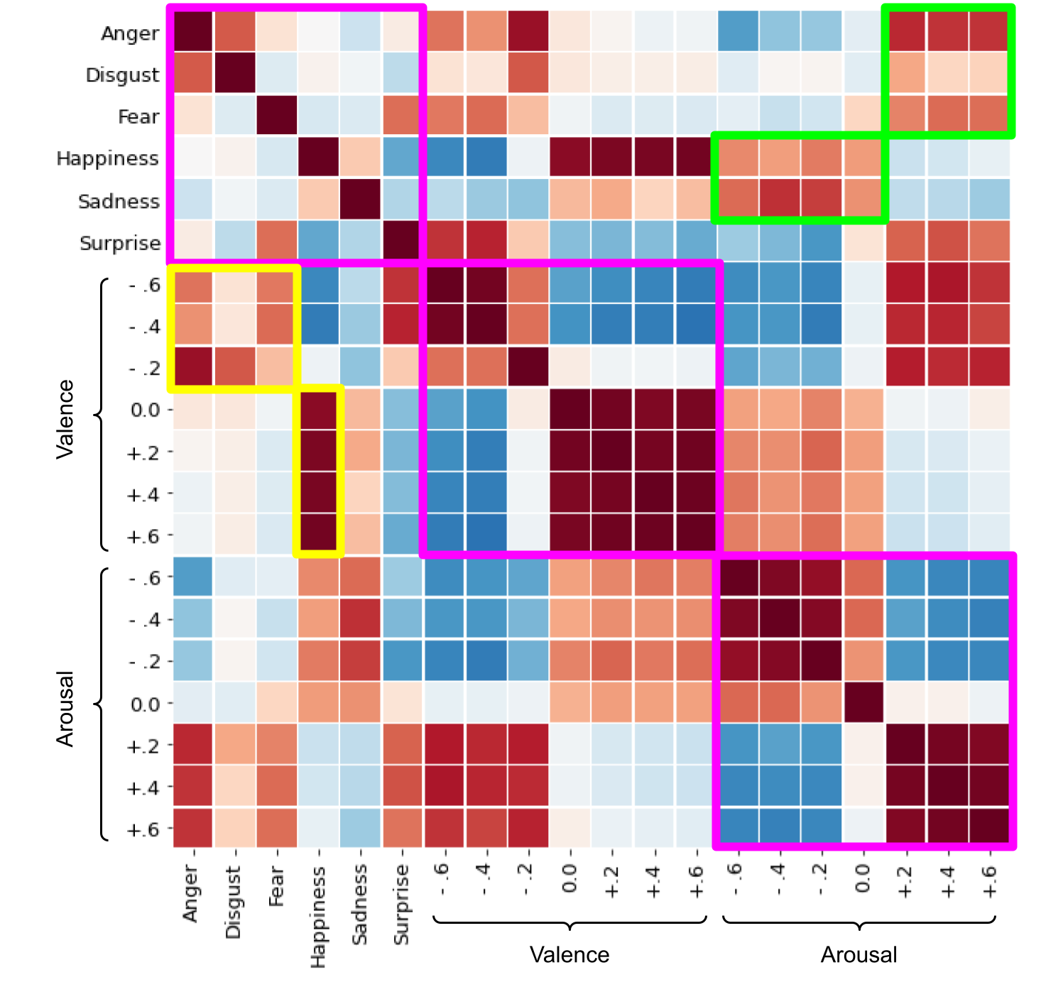
Figure F.8: Correlations between dynamic categorical emotion, valence, and arousal reconstructions. The different affective properties are delineated by the magenta borders. The green boxes highlight noteworthy correlations between high and low arousal and negative emotions (anger, disgust, and fear) and happiness/sadness, respectively. The yellow borders highlight the noteworthy correlations between positive and negative valence and happiness and negative emotions (anger, disgust, and fear), respectively.
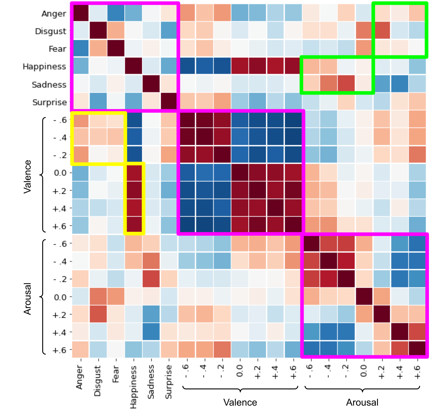
Figure F.9: Correlations between static categorical emotion, valence, and arousal reconstructions. The different affective properties are delineated by the magenta borders. The green boxes highlight noteworthy correlations between high and low arousal and negative emotions (anger, disgust, and fear) and happiness/sadness, respectively. The yellow borders highlight the noteworthy correlations between positive and negative valence and happiness and negative emotions (anger, disgust, and fear), respectively.