B Supplement to Chapter 3

The following supplementary methods describe the methods for the additional analyses done related to controlling for confounds in decoding analyses of (simulated) fMRI data and the validation of using linear confound models for brain size. All code for these simulations, analyses, and results for the fMRI-related sections can be found in functional_MRI_simulation.ipynb notebook. The code for the validation of linear confound models can be found in the notebook empirical_analysis_gender_classification.ipynb. Both notebooks are stored in the project’s Github repository (https://github.com/lukassnoek/MVCA).

B.1 Supplementary methods

B.1.1 Functional MRI simulation

B.1.1.1 Rationale

The simulations of fMRI data as described here are meant to test the efficacy of our proposed methods for confound control (CVCR) and those proposed by others (“Control for confounds during pattern estimation”; Woolgar et al., 2014) when applied to fMRI data instead of structural MRI data, as we did in the main text. One reason to suspect differences in how these methods behave between structural and functional MRI data is that we need to estimate the feature patterns ($X$) from time series for fMRI data while the feature patterns in structural MRI data are readily available. Moreover, samples in pattern analyses of fMRI data are often correlated (due to temporal autocorrelation in the fMRI signal) while it is reasonable to believe that structural MRI yields independent samples (often individual subjects).

B.1.1.2 Generation of the data ($X$, $y$, $C$)

In these simulations, we generated fMRI time series data across a grid of “voxels” ($K$) which may or may not activate in trials from different conditions. Additionally, we allow for the additive influence of a confounding variable with a prespecified correlation to the target variable (corresponding to the “additive” model from Woolgar et al., 2014). In short, we generate voxel signal ($s$) as a function of both true effects of the trials from different conditions ($\beta_{X}$), the effect of the confound ($\beta_{C}$), and autocorrelated noise ($\epsilon$):

\[\begin{equation} s = X\beta_{X} + C\beta_{C} + \epsilon, \epsilon \sim \mathcal{N}(0, V) \end{equation}\]

where $V$ specifies the covariance matrix of a signal autocorrelated as described by to an AR(1) process (we use $\phi_{1} = 0.5$). Note that, here, $X$ and $C$ refer to time-varying (HRF-convolved) predictors instead of, as in in the main text, arrays of features (voxels) across different samples. In this simulation, we evaluate two types of MVPA approaches. In the first approach, which we call “trial-wise decoding”, an activity pattern is estimated for each trial separately using the least-squares all technique (LSA; Abdulrahman & Henson, 2016). In LSA, each trial gets its own regressor in a first-level GLM. This approach is often used when there is only a single fMRI run available. In the second approach, which we call “run-wise decoding”, an activity pattern is estimated for each condition separately. Now, suppose one acquires a single run with two conditions and twenty trials per condition. In the trial-wise decoding approach, one would estimate the patterns of 40 trials (twenty for condition 1 and twenty for condition 2). Alternatively, suppose that one acquires ten runs with two conditions and again twenty trials per run. In the run-wise decoding approach, one would estimate in total twenty patterns (ten for condition 1 and ten for condition 2).

Formally, for $I$ trials across $P$ conditions, $X$ is ultimately of shape $T$ (timepoints) $\times (I \times P + 1)$ in the trial-wise decoding approach and $T \times (P+1)$ in the run-wise decoding approach (the $+ 1$ refers to the addition of an intercept). In our trial-wise simulations, we simulate 40 trials ($I$) across 2 conditions ($P$). In our run-wise simulations, we simulate 40 trials across 2 conditions in 10 runs. Note that the length of the fMRI run is automatically adjusted to the number of trials ($I$), conditions ($P$), trial duration, and interstimulus interval (ISI); increasing any of these parameters will increase the length of the run. We use a trial duration of 1 second and a jittered ISI between 4 and 5 seconds (mean = 4.5 seconds).

The initial (non-HRF-convolved) confound ($C$, with shape $N \times 1$) is generated with a prespecified correlation to the target ($y$) by adding noise ($\epsilon$) drawn from a standard normal distribution multiplied by a scaling factor ($\gamma$):

\[\begin{equation} C = y + \gamma\epsilon \end{equation}\]

This process starts with a very small scaling factor ($\gamma$). If the correlation between the target and the confound is too high, the scaling factor is increased and the process is repeated, which is iterated until the desired correlation has been found. The confound is then scaled from 0 to 1 using min-max scaling. After scaling, similar to the single-trial regressors ($X_{j}$), the confound ($C$) is also convolved with an HRF (the SPM default), representing a regressor which is parametrically modulated by the value of the confound for each trial (which could represent, for example, reaction time). The confound, $C$, now represents a time-varying array of shape $T \times 1$. This process is identical for the trial-wise and run-wise decoding approaches. However, when evaluating the efficacy of confound regression (as explained in the next section) in the context of run-wise decoding, we used the means per condition of the confound instead of the trial-wise confound values.

The simulation draws the true activation parameters for the trials from different conditions ($y \in \{0,1\}$ for $P=2$) from a normal distribution with a specified mean and standard deviation. To generate null data (i.e., without any true difference across, e.g., two conditions), we generate the true parameters as follows:

\[\begin{equation} \beta_{X(y = p)} \sim \mathcal{N}(\mu, \sigma) \end{equation}\]

where, in the case of null data, $\mu$ represents the same mean for all conditions $p = 0, \dots , P-1$. The weight of the confound ($\beta_{C}$) is also drawn from a normal distribution with a prespecified mean ($\mu_{C}$) and standard deviation ($\sigma_{C}$):

\[\begin{equation} \beta_{C} \sim \mathcal{N}(\mu_{C}, \sigma_{C}) \end{equation}\]

The weights for both $X$ and $C$ are drawn independently for the $K$ voxels (we use $10 \times 10 = 100$ voxels for all our simulations). However, to simulate spatial autocorrelation in our grid of artificial voxels, we smooth all $T$ 2D “volumes” (of shape $\sqrt{K} \times \sqrt{K}$) separately with a 2D Gaussian smoothing kernel with a prespecified standard deviation. For our simulations, we use a standard deviation of 1 for the kernel.

B.1.1.3 Estimating activity patterns from the data

After generating the signals ($s$) of shape $T \times K$ (in which the 2D voxel dimension has been flattened to a single dimension), the “activity” parameters ($\hat{\beta}_{X}$) for the trials (for trial-wise decoding) or conditions (for run-wise decoding) are estimated across all K voxels. We estimate these parameters using a generalized least squares (GLS) model on $y$ using the design matrix $X$ and covariance matrix $V$:

\[\begin{equation} \hat{\beta}_{X} = (X^{T}V^{-1}X)^{-1}X^{T}V^{-1}y \end{equation}\]

where $\hat{\beta}_{X}$ is of shape $N \times K$ (where $N$ refers to the amount of trials in trial-wise decoding and the amount of conditions in run-wise decoding). Note that $C$ is not part of the design matrix $X$, here. This would amount to the “control for confounds during pattern estimation” discussed in Supplementary Methods section “Controlling for confounds during pattern estimation”. Before entering these activity estimates ($\hat{\beta}_{X}$) in our decoding pipeline, we divide these them by their standard error to generate $t$-values (as advised in Misaki et al., 2010):

\[\begin{equation} t_{\hat{\beta}_{X}} = \frac{\hat{\beta}_{X}}{\sqrt{\sigma^{2}\mathrm{diag}(X^{T}V^{-1}X)^{-1}}} \end{equation}\]

where $\sigma^{2}$ is the sum-of-squares error divided by the degrees of freedom ($T-N-1$).

To summarize, in all of our simulations, we keep the following “experimental” parameters constant: we simulate data from two conditions ($y \in \{0,1\}$, which we refer to as “condition 0” and “condition 1”), each condition has 40 trials, trial duration is 1 second, ISIs are jittered between 4 and 5 seconds (mean = 4.5), noise is autocorrelated according to an AR(1) process (with $\phi_{1} = 0.5)$, and the data is spatially smoothed using a Gaussian filter with a standard deviation of 2 across a $10 \times 10$ grid of voxels. For run-wise decoding, we simulate 10 runs.

B.1.2 Testing confound regression on simulated fMRI data

In this simulation, we aim to test whether confound regression is able to remove the influence of confounds in fMRI data for both trial-wise and run-wise decoding analyses. Similar to the analyses reported in the main article, we contrast WDCR and CVCR, expecting that WDCR leads to similar negative bias while CVCR leads to similar (nearly) unbiased results. We use the same pipeline as in the other simulations, which consists of a normalization step to ensure that each feature has a mean of zero and a unit standard deviation, and a support vector classifier with a linear kernel (regularization parameter $C=1$). The decoding pipeline uses a 10-fold stratified cross-validation scheme. For the run-wise decoding analyses, this is equivalent to a leave-one-run-out cross-validation scheme. Model performance in this simulation is reported as accuracy (as there is no class imbalance). The simulation was repeated 10 times for robustness.

Specifically, we evaluate and report model performance after confound regression both in the trial-wise decoding and run-wise decoding context and for different strengths of the correlation between the target and the confound ($r_{Cy} \in \{0,0.1, \dots ,0.9,1\}$). Because arguably the temporal autocorrelation of fMRI data is the most prominent difference between fMRI and structural MRI data, and thus might impact decoding analyses differently (Gilron et al., 2016), we additionally test CVCR on data that differs in the degree of autocorrelation. We manipulate autocorrelation by temporally smoothing the signals ($y$) before fitting the first-level GLM using a Gaussian filter with increasing widths ($\sigma_{\mathrm{filter}} = \{0, 1 , \dots , 5\}$), yielding data with increasing autocorrelation. We used a grid of $4 \times 4$ voxels for this simulation to reduce computation time.

B.1.3 Controlling for confounds during pattern estimation

As discussed in the main text, one way to potentially control for confounds in fMRI data is to remove their influence when estimating the activity patterns in an initial first-level model (Woolgar et al., 2014). In this section of the Supplementary methods, we tested the efficacy of this method on simulated fMRI data in both trial-wise decoding and run-wise decoding contexts. Note that the original article on this method (Woolgar et al., 2014) performed run-wise decoding.

Specifically, we tested whether confounds can be controlled by adding the (HRF-convolved) confound to the design matrix $X$ in the first-level pattern estimation procedure. According to Woolgar et al. (2014), when assuming that the confound has a truly additive effect, adding the confound to the design matrix will yield (single-trial) pattern estimates ($\hat{\beta}_{X}$X) that only capture unique variance (i.e., no variance related to the confound). In our simulations, we tested two versions of this method. In one version, which we call the “default” version, the confound is added to the design matrix and the (GLS) model is estimated on using the design-matrix including both the single-trial (for trial-wise decoding) or condition regressors (for run-wise decoding) and the confound regressor. In the other version, which we call the “aggressive” version (reflecting the same terminology as the fMRI-denoising method “ICA-AROMA”; Pruim et al., 2015), the confound regressor is first regressed out of the signal ($s_{\mathrm{corr}} = s- C\hat{\beta}_{C}$) before fitting the regular first-level model using the design matrix ($X$) without the confound regressor. The reason for testing these two methods is because it is unclear from the original Woolgar et al. articles (Woolgar et al., 2011, 2014) which version was used and whether the two versions yield different results.

In our simulation, we varied the correlation between the (non-HRF-convolved) confound and the target (here, $y \in \{0,1\}$). Importantly, we generated data without any effect, i.e., the parameters of the trials from the two different conditions ($\beta_{X | y = 0}$ and $\beta_{X | y = 1}$) were (independently) drawn from the same normal distribution with a mean of 1 and standard deviation of 0.5. Similar to the other simulations, we use patterns of t-values in our decoding pipeline (unless explicitly stated otherwise). For both trial-wise and run-wise decoding, we report results from the default and aggressive procedure. All analyses are documented in the aforementioned notebook containing the fMRI simulations.

B.1.4 Linear vs nonlinear confound models: predicting VBM and TBSS data based on brain size

In the main text, we used linear models to regress out variance associated with brain size from VBM and TBSS data. Here, we test whether a linear model of the relation between brain size and VBM and TBSS data is suitable, and whether possibly a nonlinear model should have been preferred. We do this by performing a model comparison between linear, quadratic, and cubic regression models. All analyses and results can be found in the brain_data_vs_brainsize.ipynb notebook from the Github repository associated with this article.

For all analyses in this section, brain size with and without second and third degree polynomials were used as independent variables. As target variables, we created four voxel sets: first, we selected 500 random voxels from the VBM and TBSS data (voxel set A). Second, to inspect how large the misfit of a linear model could be, we selected as target variables the 500 voxels which have the highest quadratic (voxel set B) and cubic (voxel set C) correlation with brain size. Finally we select the 500 voxels with highest linear correlation with brain size (voxel set D), to inspect how large the misfit of a polynomial model is in these voxels.

We applied a 10-fold cross-validation pipeline which consisted of scaling features to mean 0 and standard deviation 1, and fitting an ordinary least squares regression model. Explained variance ($R^2$) was used as a metric of model performance. The pipeline was repeated 50 times with random shuffling of samples.

For each voxel, we calculated the difference between model performance of linear and polynomial models. Negative differences ($\Delta R^2_{\mathrm{linear - polynomial}} < 0$) indicate that the polynomial model has higher cross-validated $R^2$ than a linear model, and thus, that a linear confound regression model would leave variance arguably associated with the confound in the target voxel. We plot the distributions of $\Delta R^2_{\mathrm{linear - polynomial}}$ to inspect for how many voxels this is the case, and for how many voxels linear models perform better.

B.2 Supplementary results

The following supplementary results describe the results from the supplementary analyses related to controlling for confounds in decoding analyses of (simulated) fMRI data.

B.2.1 Testing confound regression on simulated fMRI data

Here, we evaluated the efficacy of confound regression (both WDCR and CVCR) on simulated fMRI data in both trial-wise and run-wise decoding analyses across different strengths of the correlation between the target and the confound. Similar to the results reported in the main article, we find that WDCR yields consistent below chance accuracy in both the trial-wise and run-wise decoding analyses (Supplementary Figure B.1, upper panels) and that CVCR yields (nearly) unbiased results for both trial-wise and run-wise decoding (Supplementary Figure B.1, lower panels).

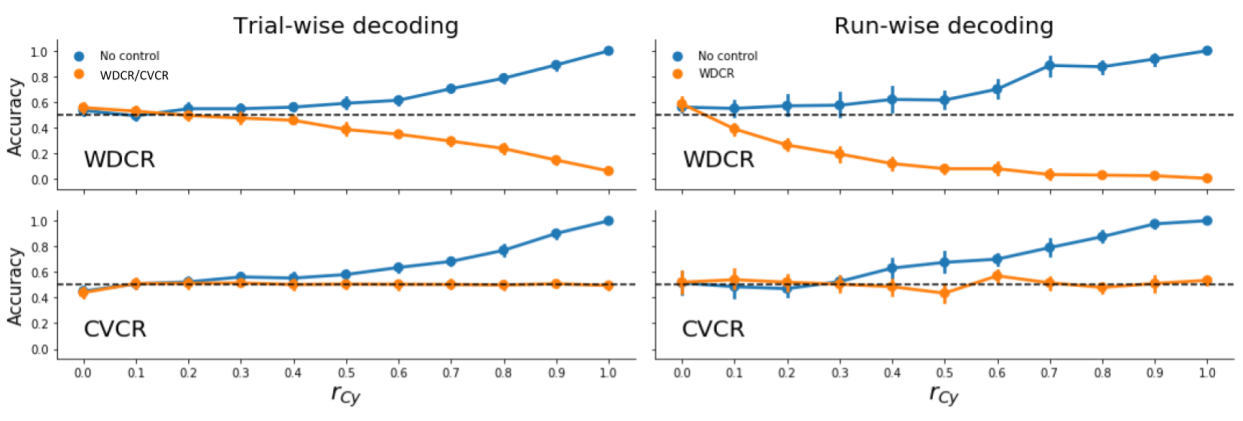
$Model performance when using WDCR (upper panels) and CVCR (lower panels) to remove the influence of confounds in simulated fMRI data across different correlations between the confound and the target ($r_{Cy}$). Error-bars reflect the 95% CI across iterations.$

Figure B.1: Model performance when using WDCR (upper panels) and CVCR (lower panels) to remove the influence of confounds in simulated fMRI data across different correlations between the confound and the target ($r_{Cy}$). Error-bars reflect the 95% CI across iterations.

Moreover, CVCR effectively controls for confounds on fMRI data with varying amounts of autocorrelation for both trial-wise and run-wise decoding analyses, as is shown in Supplementary Figure B.2.

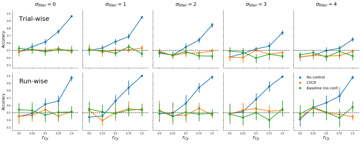
$Model performance using CVCR versus no control and baseline (data with no confound) for different levels of autocorrelation (after smoothing with a Gaussian filter with an increasing standard deviation, $\sigma_{\mathrm{filter}}$) for trial-wise and run-wise decoding. Note that for trial-wise decoding, high autocorrelation leads to below chance-accuracy for CVCR, but this is also present in the baseline data, which suggests that high autocorrelation in general leads to negative bias (at least in our simulation).$

Figure B.2: Model performance using CVCR versus no control and baseline (data with no confound) for different levels of autocorrelation (after smoothing with a Gaussian filter with an increasing standard deviation, $\sigma_{\mathrm{filter}}$) for trial-wise and run-wise decoding. Note that for trial-wise decoding, high autocorrelation leads to below chance-accuracy for CVCR, but this is also present in the baseline data, which suggests that high autocorrelation in general leads to negative bias (at least in our simulation).

B.2.2 Controlling for confounds during pattern estimation

Here, we tested the efficacy of controlling for confound during pattern estimation (as proposed by Woolgar et al., 2014). Similar to the previous Supplementary analyses, we evaluated this method’s efficacy in both trial-wise and run-wise decoding analyses. We furthermore evaluated both the “default” (add the confound to the first-level design matrix) and “aggressive” (regress the confound from the signal before fitting the first-level model) approaches.

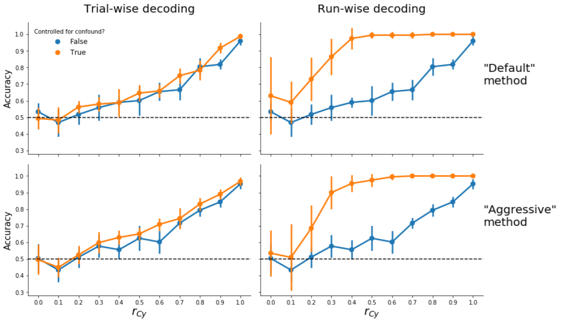
Model performance when controlling for confounds during pattern estimation using the “default” (upper panels) and “aggressive” (lower panels) versions for both trial-wise (left panels) and run-wise decoding (right panels). Note that, in these analyses, patterns of t-values from the first-level model are used as features.

Figure B.3: Model performance when controlling for confounds during pattern estimation using the “default” (upper panels) and “aggressive” (lower panels) versions for both trial-wise (left panels) and run-wise decoding (right panels). Note that, in these analyses, patterns of t-values from the first-level model are used as features.

As can be seen in Supplementary Figure B.3, this method fails to control for confounds for all variants that are tested (trial-wise vs. run-wise decoding, “default” vs. "aggressive|). Below, we provide a potential explanation of this bias. We argue that the mechanism underlying this bias is different in trial-wise decoding than in run-wise decoding. We will first focus on the trial-wise decoding analyses.

B.2.2.1 Explanation for bias in trial-wise decoding analyses

To supplement this explanation, in Supplementary Figure B.4 we visualized the distribution of parameter estimates from the first-level model, $\hat{\beta}_{X}$ across the two conditions after controlling for the confound during pattern estimation using the “aggressive” version in trial-wise decoding (but the graphs are similar when plotting the data from the “default” version; graphs for run-wise decoding analyses are, however, different, which will be discussed later).

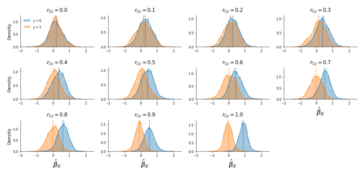
$Distribution of first-level parameter estimates, $\hat{\beta}_{X}$, for the two conditions (condition 0 in blue, condition 1 in orange) across different correlations between the target and the confound ($r_{Cy}$), with the colored dashed lines indicating the mean feature value for each condition.$

Figure B.4: Distribution of first-level parameter estimates, $\hat{\beta}_{X}$, for the two conditions (condition 0 in blue, condition 1 in orange) across different correlations between the target and the confound ($r_{Cy}$), with the colored dashed lines indicating the mean feature value for each condition.

When inspecting Supplementary Figure B.4, recall that the data were generated with a confound that was positively correlated with the target. Given that the target variable represents the two different conditions ($y \in \{0, 1\}$), the existence of a positive correlation between the target and the confound implies that the confound increases the activation of the voxel in trials from condition 0. The confound’s effect on the voxel increases with higher correlations between the target and the confound. For example, suppose trials from condition 0 and condition 1 both truly activate the voxel with 1 unit ($\beta_{X | y=0} = 1$ and $\beta_{X | y = 1} = 1$; Supplementary Figure B.5, upper panel), and that the confound is perfectly correlated with the target ($r_{Cy} = 1$) and thus activates the voxel additionally with 1 unit ($\beta_{C} = 1$). In this case, without confound control, one would expect the voxel to be activated in response to trials from condition 1 with a magnitude of 2 ($\hat{\beta}_{X | y = 1} \approx \beta_{X | y = 1} + \beta_{C}$; Supplementary Figure B.5, middle panel). If one in fact would control for the confound by regressing out the confound from the signal (i.e., the “aggressive” approach), one would completely remove both the true effect ($\beta_{X|y=1}$) and the confound effect ($\beta_{C}$), driving the estimated activation parameter for condition 1 towards 0 ($\hat{\beta}_{X|y=1} \approx 0$). The activation parameter for condition 0 is unaffected by removing the confound, as they are uncorrelated, and will thus be estimated correctly ($\hat{\beta}_{X|y=0} = 1$; see Supplementary Figure B.5, lower panel). In this way, controlling for the confound created an artificial “effect”: trials from condition 0 seem to activate the voxel more than trials from condition 1 ($\hat{\beta}_{X|y=0} > \hat{\beta}_{X|y=1}$). We believe that this phenomenon underlies the positive bias when controlling for confounds during pattern estimation in trial-wise decoding analyses.²⁰

$Visualization of the issue underlying positive bias arising when controlling for confounds during pattern estimation. The upper panel (“true generative model”) shows the individual single-trial regressors for the different conditions, scaled by their true weight (here,$\beta_{X|y=0} = \beta_{X|y=1} = 1$) and the confound (here, $r_{Cy} = 0.9$). The middle panel (“signal”) shows the signal resulting from the generative model (including noise, $\epsilon$). The lower panel (“estimated parameters”) shows the estimated model parameters for the different single-trial regressors. The dashed lines represent the average estimated parameter per condition, which shows that the estimated parameters of the condition that is correlated with the confound are driven towards zero.$

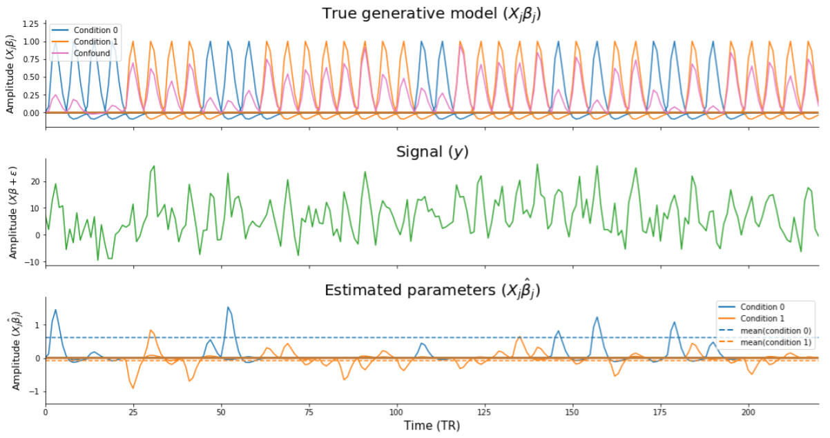
Figure B.5: Visualization of the issue underlying positive bias arising when controlling for confounds during pattern estimation. The upper panel (“true generative model”) shows the individual single-trial regressors for the different conditions, scaled by their true weight (here,$\beta_{X|y=0} = \beta_{X|y=1} = 1$) and the confound (here, $r_{Cy} = 0.9$). The middle panel (“signal”) shows the signal resulting from the generative model (including noise, $\epsilon$). The lower panel (“estimated parameters”) shows the estimated model parameters for the different single-trial regressors. The dashed lines represent the average estimated parameter per condition, which shows that the estimated parameters of the condition that is correlated with the confound are driven towards zero.

B.2.2.2 Explanation for bias in run-wise decoding analyses

We believe that the cause of bias in run-wise decoding analyses after controlling for confounds during pattern estimation is different than the cause of bias in trial-wise decoding analyses. Upon further inspection of the results of this simulation, we found that in the specific case of run-wise decoding with the “default” approach (i.e., including the confound in the first-level model instead of regressing the confound out of the signal before fitting the first-level model), there is no bias when using patterns of parameter estimates ($X$) instead of patterns of t-values (t($X$); Supplementary Figure B.6, upper row, left panel). Indeed, when visualizing the distributions of the feature values (Supplementary Figure B.6, lower row), using the “raw” parameter estimates ($\hat{\beta}_{X}$, left column) or t-values (right column), it is clear that the bias only arises when using t-values. In fact, this bias in t-values is caused by unequal variance (Supplementary Figure B.6, middle panel) of the parameter estimates. The cause of the increased variance for condition 1, here, is due to the fact that a positive correlation between the confound and target ($r_{Cy}$) results in a relatively higher correlation between the regressor of condition 1 and the confound regressor compared to the correlation between the regressor of condition 0 and the confound regressor. (Note that if the correlation would be negative, e.g., $r_{Cy} = -0.9$, then the reverse would be true.) This issue of classifiers picking up differences in parameter variance in the process of estimating patterns for MVPA has been termed “variance decoding”, which is described in detail in Görgen et al. (2017) and Hebart & Baker (2017).

$Visualization of model performance and feature distributions based on patterns of “raw” parameter estimates ($\hat{\beta}_{X}$), variance of parameter estimates ($\mathrm{var}(\hat{\beta}_{X})$), or t-values ($t(\hat{\beta}_{X})$)) after controlling for confounds. The upper row shows the average accuracy across folds across different values of the correlation between the confound and the target ($r_{Cy}$) for the different types of features. Note that the middle panel shows that “variance decoding” only occurs when controlling for confounds, as model performance is at chance when using patterns of variance estimates (the blue line in the middle panel). The lower row represents the distributions of feature values for the three different statistics when $r_{Cy} = 0.9$.$

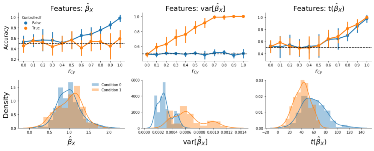
Figure B.6: Visualization of model performance and feature distributions based on patterns of “raw” parameter estimates ($\hat{\beta}_{X}$), variance of parameter estimates ($\mathrm{var}(\hat{\beta}_{X})$), or t-values ($t(\hat{\beta}_{X})$)) after controlling for confounds. The upper row shows the average accuracy across folds across different values of the correlation between the confound and the target ($r_{Cy}$) for the different types of features. Note that the middle panel shows that “variance decoding” only occurs when controlling for confounds, as model performance is at chance when using patterns of variance estimates (the blue line in the middle panel). The lower row represents the distributions of feature values for the three different statistics when $r_{Cy} = 0.9$.

To summarize, we found that controlling for confound during pattern estimation leads to positive bias in all cases except in run-wise decoding using the “default” approach. We believe that cross-validated confound regression (CVCR) is nevertheless preferable to this method because it both controls for confounds effectively and allows the use of t-values (or other statistics based on parameter estimates, like multivariate noise-normalized parameter estimates), which has been shown to be more sensitive than using “raw” parameter estimates in MVPA (Guggenmos et al., 2018; Misaki et al., 2010; Walther et al., 2016).

B.2.3 Linear vs. nonlinear confound models: predicting VBM and TBSS intensity using brain size

Supplementary Figure B.7 (top left panel) shows the distributions of difference in cross-validated $R^2$ (Linear - Polynomial) for the VBM data with 500 randomly selected voxels (voxel set A). A linear model performs (slightly) better (positive $R^2$) than a quadratic model for 86.6% of these voxels (mean $\Delta R^{2}_{\mathrm{linear-quadratic}} = 0.009$, SD = 0.006), and better than a cubic model for 90.8% of the voxels (mean $\Delta R^{2}_{\mathrm{linear-cubic}} = 0.019$, SD = 0.027). Note that it can be expected that polynomial and cubic models perform better in a minority of the voxels simply due to random noise in the data (since we compare 500 $R^2$-values), even if the “true” underlying relation is linear. To visualize the quality of fit of these models fit, brain size is plotted against VBM voxel intensity for a randomly selected voxel from this set in the bottom left panel. Lines are regression lines for the linear, quadratic, and cubic models. Supporting the use of a linear model, there is no clear deviation from bivariate normality.

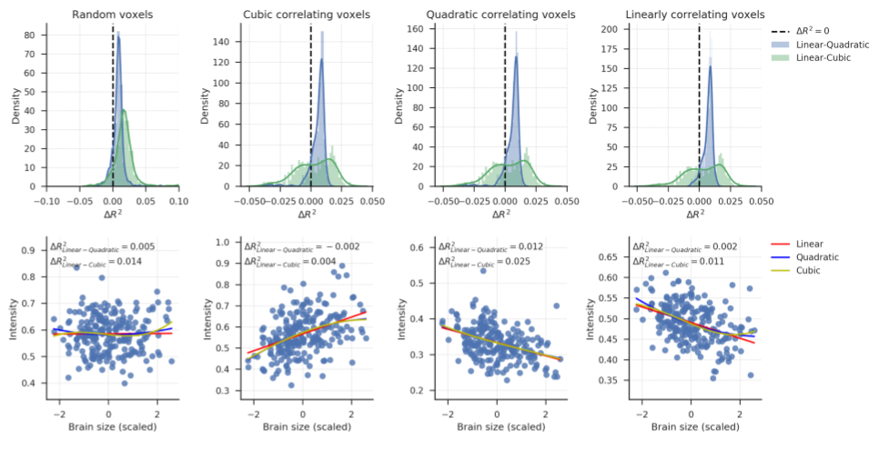
$Top row: $R^2$ distributions for the four voxel sets of the VBM data. Density estimates are obtained by kernel density estimation with a Gaussian kernel and Scott’s rule (Scott, 1979) for bandwidth selection. Bottom row: scatter plots of the relation between brain size (scaled to mean 0 and SD 1) and voxel intensity from randomly selected voxels from each voxel sets. These panels are included to visualize the quality of model fits and to inspect whether there are no obvious misfits, i.e., whether the models miss patterns in the data. This is not the case — all models seem to fit the distributions reasonably well.$

Figure B.7: Top row: $R^2$ distributions for the four voxel sets of the VBM data. Density estimates are obtained by kernel density estimation with a Gaussian kernel and Scott’s rule (Scott, 1979) for bandwidth selection. Bottom row: scatter plots of the relation between brain size (scaled to mean 0 and SD 1) and voxel intensity from randomly selected voxels from each voxel sets. These panels are included to visualize the quality of model fits and to inspect whether there are no obvious misfits, i.e., whether the models miss patterns in the data. This is not the case — all models seem to fit the distributions reasonably well.

To explore further how well linear models perform in voxels where we expect polynomial models to perform best, we plotted the $R^2$ distributions for the 500 voxels with the highest overall quadratic correlation with brain size (voxel set B; second column). These are the voxels where a quadratic model would remove most variance (if used in a confound regression procedure). Also for these voxels, a linear model performs equally well as or better than a quadratic model ($R^2_{\mathrm{linear-quadratic}} > 0$ for 89.4% of the voxels, mean $\Delta R^{2}_{\mathrm{linear-quadratic}} = 0.006$, SD = 0.007) and a cubic model ($\Delta R^{2}_{\mathrm{linear-cubic}} > 0$ for 57.8% of these voxels, mean $\Delta R^2_{\mathrm{linear-cubic}} = 0.003$, SD = 0.015). For a randomly selected voxel from this set, a scatter plot is included in the bottom panel to visualize how well the regression models fit. The plot indicates no obvious misfit of any of the models.

The same analysis was also performed for the 500 voxels that have the highest overall cubic correlation with brain size (voxel set C; third column). The histograms look similar to the histograms in the second column because voxel sets B and C consisted of largely the same voxels. It should not thus not be surprising that linear models again perform well compared to quadratic models ($\Delta R^{2}_{\mathrm{linear-quadratic}} > 0$ for 90.4% of the voxels, mean $\Delta R^2_{\mathrm{linear-quadratic}} = 0.006$, SD = 0.006), and compared to cubic models ($\Delta R^{2}_{\mathrm{linear-cubic}} > 0$ for 57.6% of these voxels, mean $\Delta R^{2}_{\mathrm{linear-cubic}} = 0.003$, SD = 0.014). The bottom panel shows a randomly selected voxel from this voxel set, which again shows no obvious misfit.

Finally, we inspect the 500 voxels with the highest overall linear correlation with brain size (voxel set D, fourth column). Again, these turned out the be partly the same voxels as in set B and C. Therefore, linear models perform again equally well as or better than quadratic models ($\Delta R^2_{\mathrm{linear-quadratic}} > 0$ for 94.2% of the voxels, mean $\Delta R^2_{\mathrm{linear-quadratic}} = 0.007$, SD = 0.004) and cubic models ($\Delta R^{2}_{\mathrm{linear-quadratic}} > 0$ for 59.2% of the voxels, mean $\Delta R^{2}_{\mathrm{linear-quadratic}} = 0.004$, SD = 0.014). The bottom panel show a randomly selected voxel from this voxel set, and indicates that all models capture the structure in the data.

Together, these results seem to imply that for all voxel sets, linear models perform mostly equally well as or better than polynomial models. Yet, it is interesting to inspect the “worst case” voxels; that is, to inspect how large the maximal misfit of a linear model is. Therefore, in Supplementary Figure B.8, we plot the relation between brain size and VBM intensity for the voxel with most negative $\Delta R^{2}_{\mathrm{linear-cubic}}$ from voxel set A (left panel) and voxel set B. For comparison, we also plot the relation between brain size and the voxel where a linear model performs better than a cubic model (selected from voxel set B). For the selected voxels, $\Delta R^{2}_{\mathrm{linear-cubic}}$ values are -0.036 (left panel), -0.039(middle panel) and 0.032. Especially in the middle and right panel, the difference in fit between the linear and cubic model is mostly apparent the tails of the brain size distribution, where the model fit is based on least observations. For most brain sizes, both models make similar predictions about voxel intensity.

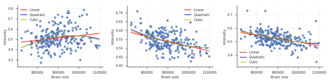
$Visualisation of the relation between brain size and VBM intensity for three voxels. The left two voxels have most negative $\Delta R^{2}_{\mathrm{linear-cubic}}$ (i.e., the cubic model performs maximally better than the linear model) in voxel sets A and B, respectively. The voxel plotted in the right panel has the most positive $\Delta R^{2}_{\mathrm{linear-cubic}}$ in voxel set B.$

Figure B.8: Visualisation of the relation between brain size and VBM intensity for three voxels. The left two voxels have most negative $\Delta R^{2}_{\mathrm{linear-cubic}}$ (i.e., the cubic model performs maximally better than the linear model) in voxel sets A and B, respectively. The voxel plotted in the right panel has the most positive $\Delta R^{2}_{\mathrm{linear-cubic}}$ in voxel set B.

We repeated the same analyses for the TBSS data, and summarize the results in Supplementary Figure B.9. Since the results are qualitatively the same as for the VBM data, and lead to the same conclusions, we do not discuss them in detail. Those interested can find additional details in the notebook of this simulation.

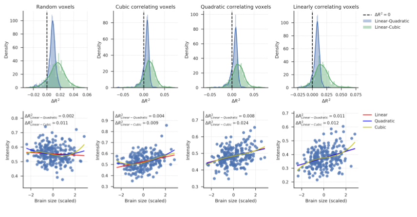
$Top row: $R^2$ distributions for the four voxel sets of the TBSS data. Density estimates are obtained by kernel density estimation with a Gaussian kernel and Scott’s rule (Scott, 1979) for bandwidth selection. Bottom row: scatter plots of the relation between brain size (scaled to mean 0 and SD 1) and voxel intensity from randomly selected voxels from each voxel sets. These panels are included to visualize the quality of model fits and to inspect whether there are no obvious misfits, i.e., whether the models miss patterns in the data. This is not the case — all models seem to fit the distributions well.$

Figure B.9: Top row: $R^2$ distributions for the four voxel sets of the TBSS data. Density estimates are obtained by kernel density estimation with a Gaussian kernel and Scott’s rule (Scott, 1979) for bandwidth selection. Bottom row: scatter plots of the relation between brain size (scaled to mean 0 and SD 1) and voxel intensity from randomly selected voxels from each voxel sets. These panels are included to visualize the quality of model fits and to inspect whether there are no obvious misfits, i.e., whether the models miss patterns in the data. This is not the case — all models seem to fit the distributions well.

$Model performance of fully cross-validated confound regression (CVCR) versus confound regression on the train-set only (“train only”) on simulated data without any experimental effect (signal $R^2 = 0.004$; left graph) and with some experimental effect (signal $R^2 = 0.1$; right graph) for different values of confound $R^2$ (cf. Figure 3.8 in the main text). The orange line represents the average performance (± 1 SD) when confound $R^2$ = 0, which serves as a “reference performance” for when there is no confounded signal in the data. For both graphs, the correlation between the target and the confound, $r_{yC}$, is fixed at 0.65. The reason for testing this version of confound regression (i.e., on the train-set only) is because it reduces the computation time substantially compared to fully cross-validated confound regression (as it does not have to compute $X_{\mathrm{test}} = X_{\mathrm{test}} - C_{\mathrm{test}}\hat{\beta}_{C}$). However, this method seems to yield substantial bias when there is (almost) no signal (left graph), but intriguingly not when there is true signal (right graph).$

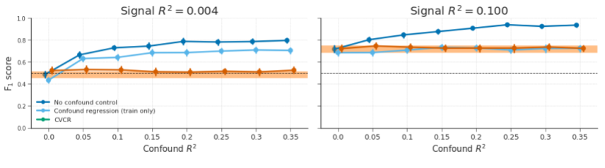
Figure B.10: Model performance of fully cross-validated confound regression (CVCR) versus confound regression on the train-set only (“train only”) on simulated data without any experimental effect (signal $R^2 = 0.004$; left graph) and with some experimental effect (signal $R^2 = 0.1$; right graph) for different values of confound $R^2$ (cf. Figure 3.8 in the main text). The orange line represents the average performance (± 1 SD) when confound $R^2$ = 0, which serves as a “reference performance” for when there is no confounded signal in the data. For both graphs, the correlation between the target and the confound, $r_{yC}$, is fixed at 0.65. The reason for testing this version of confound regression (i.e., on the train-set only) is because it reduces the computation time substantially compared to fully cross-validated confound regression (as it does not have to compute $X_{\mathrm{test}} = X_{\mathrm{test}} - C_{\mathrm{test}}\hat{\beta}_{C}$). However, this method seems to yield substantial bias when there is (almost) no signal (left graph), but intriguingly not when there is true signal (right graph).

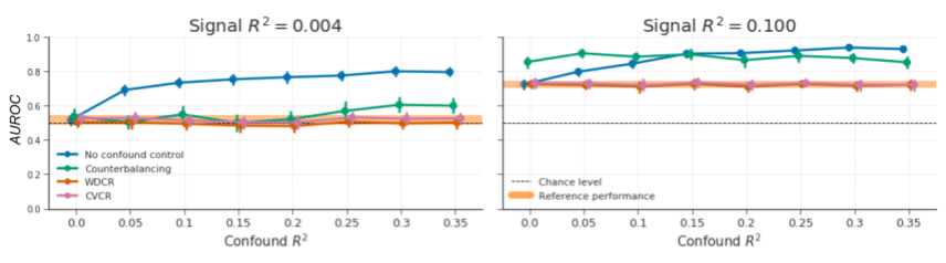
$Model performance of the different evaluated methods for confound control but using the AUC-ROC metric to measure model performance instead of $F_{1}$ score, as this latter metric has been criticized because it neglects false negatives (Powers, 2011). The results are highly similar to results obtained when using the $F_{1}$ score (cf. Figure 3.8 in the main text).$

Figure B.11: Model performance of the different evaluated methods for confound control but using the AUC-ROC metric to measure model performance instead of $F_{1}$ score, as this latter metric has been criticized because it neglects false negatives (Powers, 2011). The results are highly similar to results obtained when using the $F_{1}$ score (cf. Figure 3.8 in the main text).

Model performance of the different evaluated methods for confound control, including a method proposed by a reviewer. This method entails training the decoding model on data including the confound as a predictor (i.e., an implementation of the “Include confound in model” method), but setting the confound values to their mean in the test set. The rationale is that the decoding model cannot profit from the confound in the test set. However, contrary to expectations, this method performs similarly to not controlling for confounds.

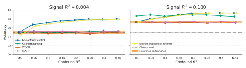
Figure B.12: Model performance of the different evaluated methods for confound control, including a method proposed by a reviewer. This method entails training the decoding model on data including the confound as a predictor (i.e., an implementation of the “Include confound in model” method), but setting the confound values to their mean in the test set. The rationale is that the decoding model cannot profit from the confound in the test set. However, contrary to expectations, this method performs similarly to not controlling for confounds.

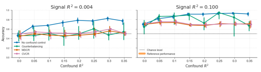
Reproduction of Figure 3.8 from the main text (“generic simulation” results), but with the random subsampling procedure instead of the targeted subsampling procedure (from only a single iteration due to time constraints). This procedure attempts to find a subsample of the data of a given size without a correlation between target and confound for 10.000 tries. If such a subsample cannot be found, the subsample size is decreased by 1, after which again 10.000 attempts are made to find a good subsample with the new size. The results from counterbalancing, here, are qualitatively similar to the results when using the “targeted subsampling” method (cf. Figure 3.8 in the main text), albeit much slower.

Figure B.13: Reproduction of Figure 3.8 from the main text (“generic simulation” results), but with the random subsampling procedure instead of the targeted subsampling procedure (from only a single iteration due to time constraints). This procedure attempts to find a subsample of the data of a given size without a correlation between target and confound for 10.000 tries. If such a subsample cannot be found, the subsample size is decreased by 1, after which again 10.000 attempts are made to find a good subsample with the new size. The results from counterbalancing, here, are qualitatively similar to the results when using the “targeted subsampling” method (cf. Figure 3.8 in the main text), albeit much slower.

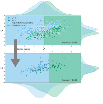
Reproduction of Figure 3.10 from the main text, but with the random subsampling procedure instead of the targeted subsampling procedure. This procedure attempts to find a subsample of the data of a given size without a correlation between target and confound for 10.000 tries. If such a subsample cannot be found, the subsample size is decreased by 1, after which again 10.000 attempts are made to find a good subsample with the new size. The plot shows that also random subsampling can induce a positive bias, even with extreme power loss (90% smaller sample).

Figure B.14: Reproduction of Figure 3.10 from the main text, but with the random subsampling procedure instead of the targeted subsampling procedure. This procedure attempts to find a subsample of the data of a given size without a correlation between target and confound for 10.000 tries. If such a subsample cannot be found, the subsample size is decreased by 1, after which again 10.000 attempts are made to find a good subsample with the new size. The plot shows that also random subsampling can induce a positive bias, even with extreme power loss (90% smaller sample).

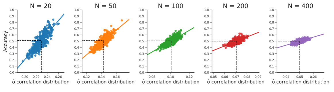
$These plots show that the relationship between the standard deviation of the empirical feature-target correlation distribution, sd($r_{yX}$), and accuracy holds for different samples sizes (i.e., values for $N$). Note that the predicted accuracy based on the standard deviation expected from the sampling distribution is at 0.5 for every plot. The data were generated in the same manner as reported in the WDCR follow-up section.$

Figure B.15: These plots show that the relationship between the standard deviation of the empirical feature-target correlation distribution, sd($r_{yX}$), and accuracy holds for different samples sizes (i.e., values for $N$). Note that the predicted accuracy based on the standard deviation expected from the sampling distribution is at 0.5 for every plot. The data were generated in the same manner as reported in the WDCR follow-up section.

These plots show that the relationship between the standard deviation of the empirical feature-target correlation distribution and accuracy also holds for sizes of the test-set (replicating results from Jamalabadi et al., 2016). Note that the predicted accuracy is again at 0.5 for every plot. The data were generated in the same manner as reported in the WDCR follow-up section.

Figure B.16: These plots show that the relationship between the standard deviation of the empirical feature-target correlation distribution and accuracy also holds for sizes of the test-set (replicating results from Jamalabadi et al., 2016). Note that the predicted accuracy is again at 0.5 for every plot. The data were generated in the same manner as reported in the WDCR follow-up section.

$These plots show that the relationship between the standard deviation of the empirical feature-target correlation distribution, sd($r_{yX}$), and accuracy also holds for different numbers of features ($K$). Note that the predicted accuracy based on sd($r_{yX}$) is approximately at 0.5 for every plot. The data were generated in the same manner as reported in the WDCR follow-up section.$

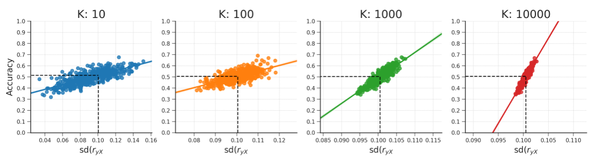
Figure B.17: These plots show that the relationship between the standard deviation of the empirical feature-target correlation distribution, sd($r_{yX}$), and accuracy also holds for different numbers of features ($K$). Note that the predicted accuracy based on sd($r_{yX}$) is approximately at 0.5 for every plot. The data were generated in the same manner as reported in the WDCR follow-up section.

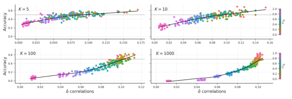
$The relation of the standard deviation of the correlation distribution and accuracy for different values of $K$.$

Figure B.18: The relation of the standard deviation of the correlation distribution and accuracy for different values of $K$.

One could argue that this issue only poses a problem when the true parameters are non-zero ($\beta_{X|y=0} = \beta_{X|y=1} \neq 0$) and when the true parameters are in fact all zero ($\beta_{X|y=0} = \beta_{X|y=1} = 0$), there would be no positive bias. This is indeed the case, but we note that the true parameters are never known in empirical anlayses, so we nonetheless advise against using this method.↩︎

Towards prediction