3 How to control for confounds in decoding analyses of neuroimaging data

This chapter has been published as: Snoek, L.*, Miletić, S.*, & Scholte, H.S. (2019). How to control for confounds in decoding analyses of neuroimaging data. NeuroImage, 184, 741-760.

* Shared first authorship

Abstract

Over the past decade, multivariate “decoding analyses” have become a popular alternative to traditional mass-univariate analyses in neuroimaging research. However, a fundamental limitation of using decoding analyses is that it remains ambiguous which source of information drives decoding performance, which becomes problematic when the to-be-decoded variable is confounded by variables that are not of primary interest. In this study, we use a comprehensive set of simulations as well as analyses of empirical data to evaluate two methods that were previously proposed and used to control for confounding variables in decoding analyses: post hoc counterbalancing and confound regression. In our empirical analyses, we attempt to decode gender from structural MRI data while controlling for the confound “brain size”. We show that both methods introduce strong biases in decoding performance: post hoc counterbalancing leads to better performance than expected (i.e., positive bias), which we show in our simulations is due to the subsampling process that tends to remove samples that are hard to classify or would be wrongly classified; confound regression, on the other hand, leads to worse performance than expected (i.e., negative bias), even resulting in significant below chance performance in some realistic scenarios. In our simulations, we show that below chance accuracy can be predicted by the variance of the distribution of correlations between the features and the target. Importantly, we show that this negative bias disappears in both the empirical analyses and simulations when the confound regression procedure is performed in every fold of the cross-validation routine, yielding plausible (above chance) model performance. We conclude that, from the various methods tested, cross-validated confound regression is the only method that appears to appropriately control for confounds which thus can be used to gain more insight into the exact source(s) of information driving one’s decoding analysis.

3.1 Introduction

In the past decade, multivariate pattern analysis (MVPA) has emerged as a popular alternative to traditional univariate analyses of neuroimaging data (Haxby, 2012; Norman et al., 2006). The defining feature of MVPA is that it considers patterns of brain activation instead of single units of activation (i.e., voxels in MRI, sensors in MEG/EEG). One of the most-often used type of MVPA is “decoding”, in which machine learning algorithms are applied to neuroimaging data to predict a particular stimulus, task, or psychometric feature. For example, decoding analyses have been used to successfully predict various experimental conditions within subjects, such as object category from fMRI activity patterns (Haxby et al., 2001) and working memory representations from EEG data (LaRocque et al., 2013), as well between-subject factors such as Alzheimer’s disease (vs. healthy controls) from structural MRI data (Cuingnet et al., 2011) and major depressive disorder (vs. healthy controls) from resting-state functional connectivity (Craddock et al., 2009). One reason for the popularity of MVPA, and especially decoding, is that these methods appear to be more sensitive than traditional mass-univariate methods in detecting effects of interest. This increased sensitivity is often attributed to the ability to pick up multidimensional, spatially distributed representations which univariate methods, by definition, cannot do (Jimura & Poldrack, 2012). A second important reason to use decoding analyses is that they allow researchers to make predictions about samples beyond the original dataset, which is more difficult using traditional univariate analyses (Hebart & Baker, 2017).

In the past years, however, the use of MVPA has been criticized for a number of reasons, both statistical (Allefeld et al., 2016; Davis et al., 2014; Gilron et al., 2017; Haufe et al., 2014) and more conceptual (Naselaris & Kay, 2015; Weichwald et al., 2015) in nature. For the purposes of the current study, we focus on the specific criticism put forward by Naselaris & Kay (2015) , who argue that decoding analyses are inherently ambiguous in terms of what information they use (see Popov et al., 2018 for a similar argument in the context of encoding analyses). This type of ambiguity arises when the classes of the to-be-decoded variable systematically vary in more than one source of information (see also Carlson & Wardle, 2015; Ritchie et al., 2017; Weichwald et al., 2015). The current study aims to investigate how decoding analyses can be made more interpretable by reducing this type of “source ambiguity”.

To illustrate the problem of source ambiguity, consider, for example, the scenario in which a researcher wants to decode gender.⁴ (male/female) from structural MRI with the aim of contributing to the understanding of gender differences — an endeavor that generated considerable interest and controversy (Chekroud et al., 2016; Del Giudice et al., 2016; Glezerman, 2016; Joel & Fausto-Sterling, 2016; Rosenblatt, 2016). By performing a decoding analysis on the MRI data, the researcher hopes to capture meaningful patterns of variation in the data of male and female participants that are predictive of the participant’s gender. The literature suggests that gender dimorphism in the brain is manifested in two major ways (Good, Johnsrude, et al., 2001 b; O’Brien et al., 2011). First, there is a global difference between male and female brains: men have on average about 15% larger intracranial volume than women, which falls in the range of mean gender differences in height (8.2%) and weight (18.7%; Gur et al., 1999; Lüders et al., 2002).⁵ Second, brains of men and women are known to differ locally: some specific brain areas are on average larger in women than in men (e.g., in superior and middle temporal cortex; Good, Johnsrude, et al., 2001 a) and vice versa (e.g., in frontomedial cortex; Goldstein et al., 2001). One could argue that, given that one is interested in explaining behavioral or mental gender differences, global differences are relatively uninformative, as it reflects the fact than male bodies are on average larger than female bodies (Gur et al., 1999; Sepehrband et al., 2018). As such, our hypothetical researcher is likely primarily interested in the local sources of variation in the neuroanatomy of male and female brains.

Now, supposing that the researcher is able to decode gender from the MRI data significantly above chance, it remains unclear on which source of information the decoder is capitalizing: the (arguably meaningful) local difference in brain structure or the (in the context of this question arguably uninteresting) global difference in brain size? In other words, the data contain more than one source of information that may be used to predict gender. In the current study, we aim to evaluate methods that improve the interpretability of decoding analyses by controlling for “uninteresting” sources of information.

3.1.1 Partitioning effects into true signal and confounded signal

Are multiple sources of information necessarily problematic? And what makes a source of information interesting or uninteresting? The answers to these questions depend on the particular goal of the researcher using the decoding analysis (Hebart & Baker, 2017). In principle, multiple sources of information in the data do not pose a problem if a researcher is only interested in accurate prediction, but not in interpretability of the model (Bzdok, 2017; Haufe et al., 2014; Hebart & Baker, 2017). In brain-computer interfaces (BCI), for example, accurate prediction is arguably more important than interpretability, i.e., knowing which sources of information are driving the decoder. Similarly, if the researcher from our gender decoding example is only interested in accurately predicting gender regardless of model interpretability, source ambiguity is not a problem.⁶ In most scientific applications of decoding analyses, however, model interpretability is important, because researchers are often interested in the relative contributions of different sources of information to decoding performance. Specifically, in most decoding analyses, researchers often (implicitly) assume that the decoder is only using information in the neuroimaging data that is related to the variable that is being decoded (Ritchie et al., 2017). In this scenario, source ambiguity (i.e., the presence of multiple sources of information) is problematic as it violates this (implicit) assumption. Another way to conceptualize the problem of source ambiguity is that, using the aforementioned example, (global) brain size is confounding the decoding analysis of gender. Here, we define a confound as a variable that is not of primary interest, correlates with the to-be-decoded variable (the target), and is encoded in the neuroimaging data.

To illustrate the issue of confounding variables in the context of decoding clinical disorders, suppose one is interested in building a classifier that is able to predict whether subjects are suffering from schizophrenia or not based on the subjects’ gray matter data. Here, the variable “schizophrenia-or-not” is the variable of interest, which is assumed to be encoded in the neuroimaging data (i.e., the gray matter) and can thus be decoded. However, there are multiple factors known to covary with schizophrenia, such as gender (i.e., men are more often diagnosed with schizophrenia than women; McGrath et al., 2008) and substance abuse (Dixon, 1999), which are also known to affect gray matter (Bangalore et al., 2008; Gur et al., 1999; Van Haren et al., 2013). As such, the variables gender and substance abuse can be considered confounds according to our definition, because they are both correlated with the target (schizophrenia or not) and are known to be encoded in the neuroimaging data (i.e., the effect of these variables is present in the gray matter data). Now, if one is able to classify schizophrenia with above-chance accuracy from gray matter data, one cannot be sure which source of information within the data is picked up by the decoder: information (uniquely) associated with schizophrenia or (additionally) information associated with gender or substance abuse? If one is interested in more than mere accurate prediction of schizophrenia, then this ambiguity due to confounding sources of information is problematic.

Importantly, as our definition suggests, what is or is not regarded as a confound is relative — it depends on whether the researchers deems it of (primary) interest or not. In the aforementioned hypothetical schizophrenia decoding study, for example, one may equally well define the severity of substance abuse as the to-be-decoded variable, in which the variable “schizophrenia-or-no”” becomes the confounding variable. In other words, one researcher’s signal is another researcher’s confound. Regardless, if decoding analyses of neuroimaging data are affected by confounds, the data thus contain two types of information: the “true signal” (i.e., variance in the neuroimaging data related to the target, but unrelated to the confound) and the “confounded signal” (i.e., variance in the neuroimaging data related to the target that is also related to the confound; see Figure 3.1). In other words, source ambiguity arises due to the presence of both true signal and confounded signal and, thus, controlling for confounds (by removing the confounded signal) provides a crucial methodological step forward in improving the interpretability of decoding analyses.

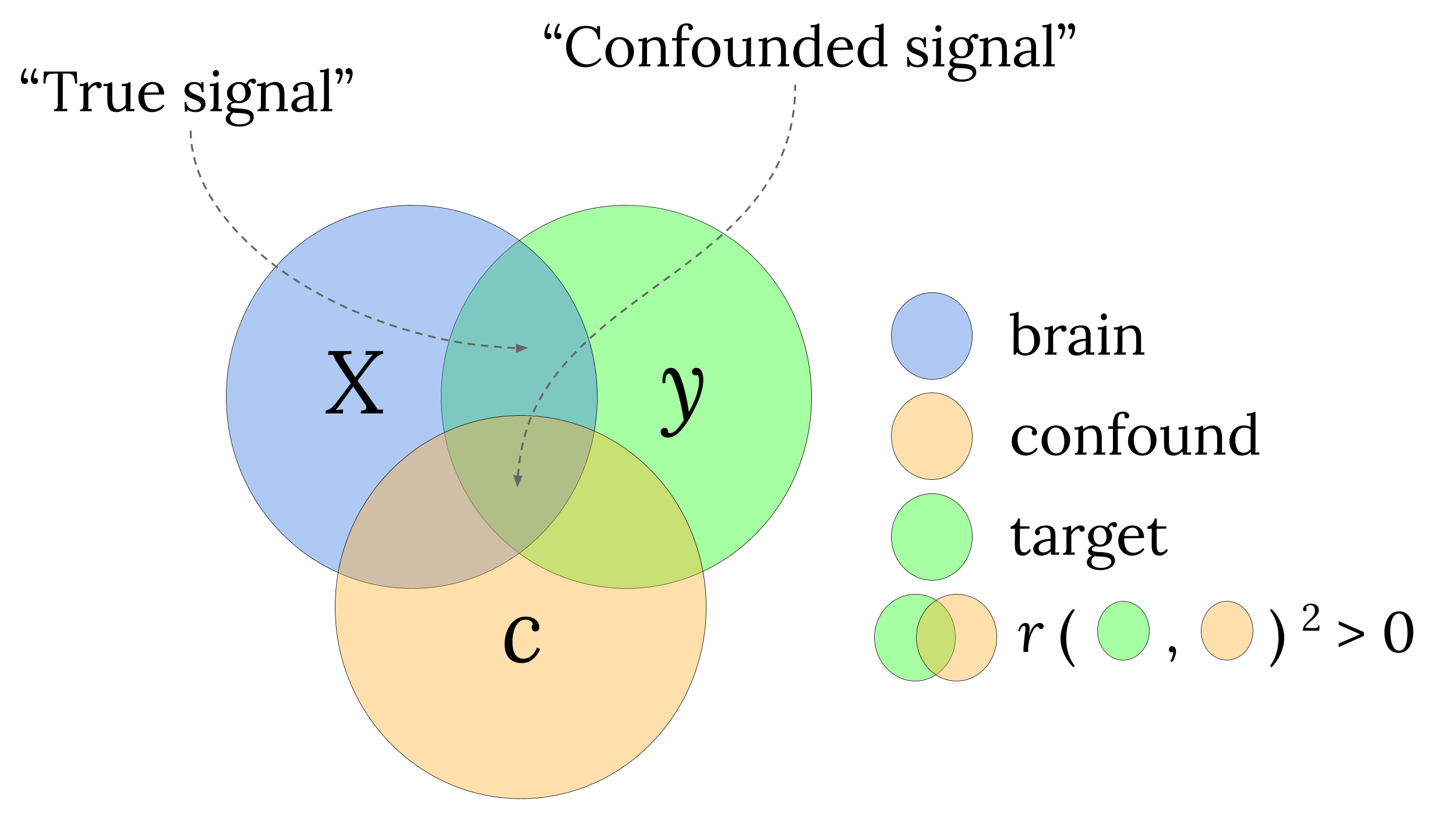
$Visualization of how variance in brain data ($X$) can partitioned into “True signal” and “Confounded signal”, depending on the correlation structure between the brain data ($X$), the confound ($C$), and the target ($y$). Overlapping circles indicate a non-zero (squared) correlation between the two variables.$

Figure 3.1: Visualization of how variance in brain data ($X$) can partitioned into “True signal” and “Confounded signal”, depending on the correlation structure between the brain data ($X$), the confound ($C$), and the target ($y$). Overlapping circles indicate a non-zero (squared) correlation between the two variables.

In the decoding literature, various methods have been applied to control for confounds. We next provide an overview of these methods, highlight their advantages and disadvantages, and discuss their rationale and the types of research settings they can be applied in. Subsequently, we focus on two of these methods to test whether these methods succeed in controlling for the influence of confounds.

3.1.2 Methods for confound control

In decoding analyses, one aims to predict a certain target variable from patterns of neuroimaging data. Various methods discussed in this section are supplemented with a mathematical formalization; for consistency and readability, we define the notation we will use in Table 3.1.

Table 3.1: Notation.
Symbol	Dims.	Description
$N$		Number of samples (usually subjects or trials)
$K$		Number of neuroimaging features (e.g., voxels or sensors)
$P$		Number of confound variables (e.g., age, reaction time, or brain size)
$X_{ij}$	$N \times K$	The neuroimaging patterns (often called the “data” in the current article), where the subescript $i \in {1 \dots N}$ refers to the individual samples (rows), and the subscript $j \in {1 \dots K}$ to individual features (columns)
$y$	$N \times 1$	The target variable (i.e., what is to be decoded)
$C$	$N \times P$	The confound variable(s)
$\hat{\beta}$	$K + 1$	The parameters estimated in a general linear model (GLM)
$w$	$K + 1$	The parameters estimated in a decoding model
$r_{Cy}$		Sample Pearson correlation coefficient between $C$ and $y$
$r_{y(X.C)}$		Sample semipartial Pearson correlation coefficient between $X$ and $y$, controlled for $C$
$p(r_{Cy})$		$p$-value of sample Pearson correlation between $C$ and $y$
Note: Format based on Diedrichsen and Kriegeskorte (2017). For the correlations ($r$), we assume that $P = 1$ and thus that the correlations in the table reduce to a scalar.

3.1.2.1 A priori counterbalancing

Ideally, one would prevent confounding variables from influencing the results as much as possible before the acquisition of the neuroimaging data.⁷ One common way do this (in both traditional “activation-based” and decoding analyses) is to make sure that potential confounding variables are counterbalanced in the experimental design (Görgen et al., 2017). In experimental research, this would entail randomly assigning subjects to design cells (e.g., treatment groups) such that there is no structural correlation between characteristics of the subjects and design cells. In observational designs (e.g., in the gender/brain size example described earlier), it means that the sample is chosen such that there is no correlation between the confound (brain size) and observed target variable (gender). That is, given that men on average have larger brains than women, this would entail including only men with relatively small brains and women with relatively large brains.⁸ The distinction between experimental and observational studies is important because the former allow the researcher to randomly draw samples from the population, while the latter require the researcher to choose a sample that is not representative of the population, which limits the conclusions that can be drawn about the population (we will revisit this issue in the Discussion section).

Formally, in decoding analyses, a design is counterbalanced when the confound $C$ and the target $y$ are statistically independent. In practice, this often means that the sample is chosen so that there is no significant correlation coefficient between $C$ and $y$ (although this does not necessarily imply that $C$ and $y$ are actually independent). To illustrate the process of counterbalancing, let’s consider another hypothetical experiment: suppose one wants to set up an fMRI experiment in which the goal is to decode abstract object category (e.g., faces vs. houses) from the corresponding fMRI patterns (cf. Haxby et al., 2001), while controlling for the potential confounding influence of low-level or mid-level stimulus features, such as luminance, spatial frequency, or texture (Long et al., 2017). Proper counterbalancing would entail making sure that the images used for this particular experiments have similar values for these low-level and mid-level features across object categories (see for details Görgen et al., 2017). Thus, in this example, low-level and mid-level stimulus features should be counterbalanced with respect to object category, such that above chance decoding of object category cannot be attributed to differences in low-level or mid-level stimulus features (i.e., the confounds).

A priori counterbalancing of potential confounds is, however, not always feasible. For one, the exact measurement of a potentially confounding variable may be impossible until data acquisition. For example, the brain size of a participant is only known after data collection. Similarly, Todd et al. (2013) found that their decoding analysis of rule representations was confounded by response times of to the to-be-decoded trials. Another example of a “data-driven” confound is participant motion during data acquisition (important in, for example, decoding analyses applied to data from clinical populations such as ADHD; Yu-Feng et al., 2007). In addition, a priori counterbalancing of confounds may be challenging because of the limited size of populations of interest. Especially in clinical research settings, researchers may not have the luxury of selecting a counterbalanced sample due to the small number of patient subjects available for testing. Lastly, researchers may simply discover confounds after data acquisition.

Given that a priori counterbalancing is not possible or undesirable in many situations, it is paramount to explore the possibilities of controlling for confounding variables after data acquisition for the sake of model interpretability, which we discuss next.

3.1.2.2 Include confounds in the data

One perhaps intuitive method to control for confounds in decoding analyses is to include the confound(s) in the data (i.e., the neuroimaging data, $X$; see, e.g., Sepehrband et al., 2018) used by decoding model. That is, when applying a decoding analysis to neuroimaging data, the confound is added to the data as if it were another voxel (or sensor, in electrophysiology). This intuition may stem from the analogous situation in univariate (activation-based) analyses of neuroimaging data, in which confounding variables are controlled for by including them in the design matrix together with the stimulus/task regressors. For example, in univariate analyses of functional MRI, movement of the participant is often controlled for by including motion estimates in the design matrix of first-level analyses (Johnstone et al., 2006); in EEG, some control for activity due to eye-movements by including activity measured by concurrent electro-oculography as covariates in the design-matrix (Parra et al., 2005). Usually, the general linear model is then used to estimate each predictor’s influence on the neuroimaging data. Importantly, the parameter estimates ($\hat{\beta}$) are often interpreted as reflecting the unique contribution⁹ of each predictor variable, independent from the influence of the confound.

Contrary to general linear models as employed in univariate (activation-based) analyses, including confound variables in the data as predictors for decoding models is arguably problematic. If a confound is included in the data in the context of decoding models, the parameter estimates of the features (often called “feature weights”, $w$, in decoding models) may be corrected for the influence of the confound, but the model performance (usually measured as explained variance, $R^2$, or classification accuracy; Hebart & Baker, 2017) is not. That is, rather than providing an estimate of decoding performance “controlled for” a confound, one obtains a measure of performance when explicitly including the confound as an interesting source of variance that the decoder is allowed to use. This is problematic because research using decoding analyses generally does not focus on parameter estimates but on statistics of model performance. Model performance statistics (e.g., $R^2$, classification accuracy) alone cannot disentangle the contribution of different sources of information as they only represent a single summary statistic of model fit (Ritchie et al., 2017). One might, then, argue that additionally inspecting feature weights of decoding models may help in disambiguating different sources of information (Sepehrband et al., 2018). However, it has been shown that feature weights cannot be reliably mapped to specific sources of information, i.e., as being task-related or confound-related (e.g., features with large weights may be completely uncorrelated with the target variable; Haufe et al., 2014; Hebart & Baker, 2017). As such, it does not make sense to include confounds in the set of predictors when the goal is to disambiguate the different sources of information in decoding analyses.

Recently, another approach similar to including confounds in the data has been proposed, which is based on the idea of a dose-response curve (Alizadeh et al., 2017). In this method, instead of adding the confound(s) to the model directly, the relative contribution of true and confounded signal is systematically controlled. The authors show that this approach is able to directly quantify the unique contribution of each source of information, thus effectively controlling for confounded signal. However, while sophisticated in its approach, this method only seems to work for categorical confounds, as it is difficult (if not impossible) to systematically vary the proportion of confound-related information when dealing with continuous confounds or when dealing with more than one confound.

3.1.2.3 Control for confounds during pattern estimation

Another method that was used in some decoding studies on functional MRI data aims to control for confounds in the initial procedure of estimating activity patterns of the to-be-decoded events, by leveraging the ability of the GLM to yield parameter estimates reflecting unique variance (Woolgar et al., 2014). In this method, an initial “first-level” (univariate) analysis models the fMRI time series ($s$) as a function of both predictors-of-interest ($X$) and the confounds ($C$), often using the GLM¹⁰:

\[\begin{equation} s = X\beta_{x} + C\beta_{c} + \epsilon \end{equation}\]

Then, only the estimated parameters ($\hat{\beta}$, or normalized parameters, such as t-values or z-values) corresponding to the predictors-of-interest ($\hat{\beta}_{x}$) are used as activity estimates (i.e., the used for predicting the target $y$) in the subsequent decoding analyses. This method thus takes advantage of the shared variance partitioning in the pattern estimation step to control for potential confounding variables. However, while elegant in principle, this method is not applicable in between-subject decoding studies (e.g., clinical decoding studies; Waarde et al., 2014; Cuingnet et al., 2011), in which confounding variables are defined across subjects, or in electrophysiology studies, in which activity patterns do not have to be¹¹ estimated in a first-level model, thus limiting the applicability of this method.

3.1.2.4 Post hoc counterbalancing of confounds

When a priori counterbalancing is not possible, some have argued that post hoc counterbalancing might control for the influence of confounds (Rao et al., 2017, pp. 24, 38). In this method, given that there is some sample correlation between the target and confound ($r_{Cy} \neq 0$) in the entire dataset, one takes a subset of samples in which there is no empirical relation between the confound and the target (e.g., when $r_{Cy} \approx 0$). In other words, post hoc counterbalancing is a way to decorrelate the confound and the target by subsampling the data. Then, subsequent decoding analysis on the subsampled data can only capitalize on true signal, as there is no confounded signal anymore (see Figure 3.2). While intuitive in principle, we are not aware of whether this method has been evaluated before and whether it yields unbiased performance estimates.

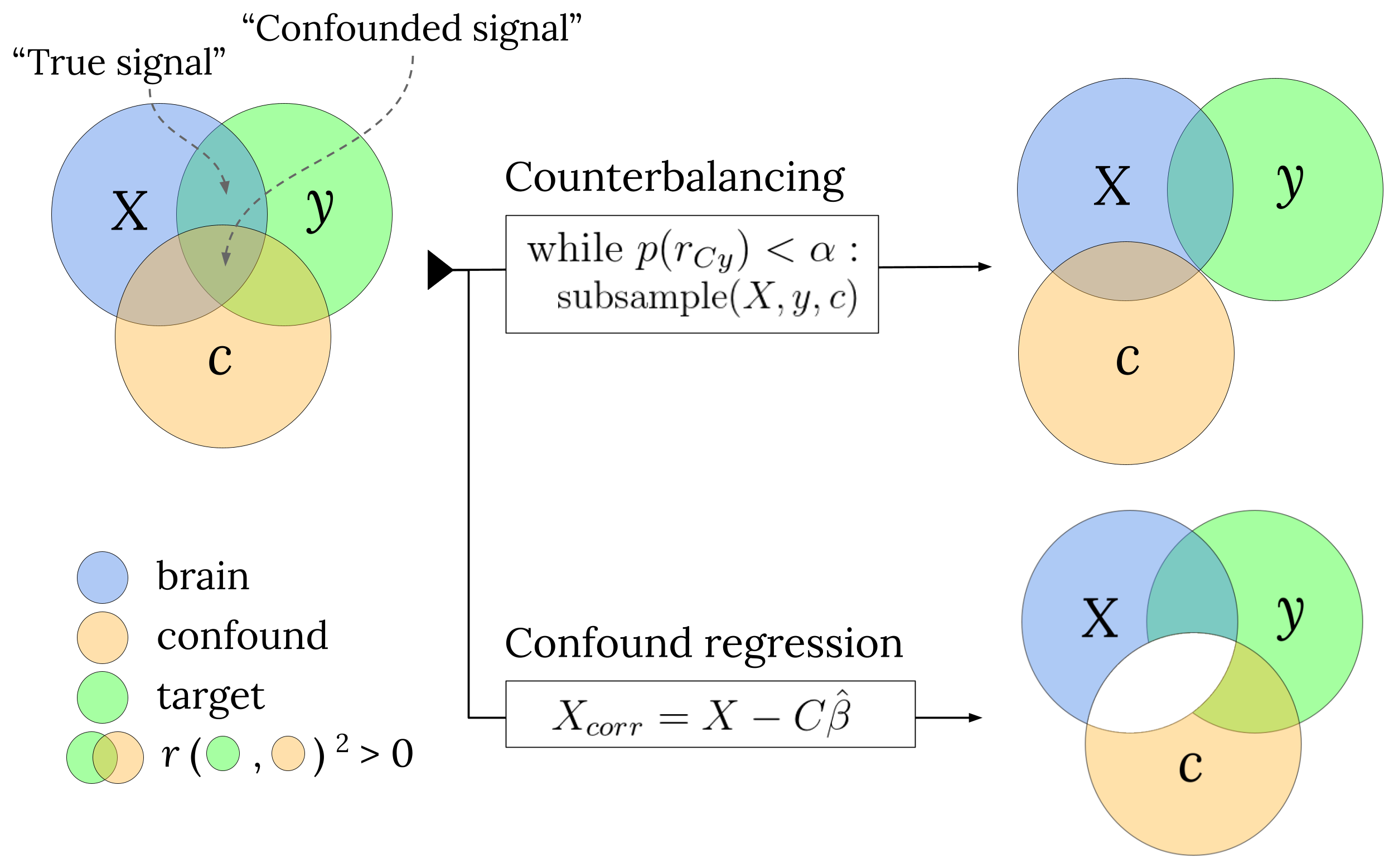
A schematic visualization how the main two confound control methods evaluated in this article deal with the “confounded signal”, making sure decoding models only capitalize on the “true signal”.

Figure 3.2: A schematic visualization how the main two confound control methods evaluated in this article deal with the “confounded signal”, making sure decoding models only capitalize on the “true signal”.

3.1.2.5 Confound regression

The last and perhaps most common method to control for confounds is removing the variance that can be explained by the confound (i.e., the confounded signal) from the neuroimaging data directly (Abdulkadir et al., 2014; Dukart et al., 2011; Kostro et al., 2014; Rao et al., 2017; Todd et al., 2013) — a process we refer to as confound regression (also known as “image correction”; Rao et al., 2017). In this method, a (usually linear) regression model is fitted on each feature in the neuroimaging data (i.e., a single voxel or sensor) with the confound(s) as predictor(s). Thus, each feature in the neuroimaging data $X$ is modelled as a linear function of the confounding variable(s), $C$:

\[\begin{equation} X_{j} = C\beta + \epsilon \end{equation}\]

We can estimate the parameter(s) for feature using, for example, ordinary least squares as follows (for an example using a different model, see Abdulkadir et al., 2014):

\[\begin{equation} \hat{\beta}_{j} = (C^{T}C)^{-1}C^{T}X_{j} \end{equation}\]

Then, to remove the variance of (or “regress out”) the confound from the neuroimaging data, we can subtract the variance in the data associated with confound ($C\hat{\beta}_{j}$) from the original data:

\[\begin{equation} X_{j,\mathrm{corr}} = X_{j} - C\hat{\beta}_{j} \end{equation}\]

In which $X_{j,\mathrm{corr}}$ represents the neuroimaging feature $X_{j}$ from which all variance of the confound is removed (including the variance shared with $y$, i.e., the confounded signal; see Figure 3.2). When subsequently applying a decoding analysis on this corrected data, one can be sure that the decoder is not capitalizing on signal that is correlated with the confound, which thus improves interpretability of the decoding analysis.

Confound regression has been applied in several decoding studies. Todd et al. (2013) were, as far as the current authors are aware, the first to use this method to control for a confound (in their case, reaction time) that was shown to correlate with their target variable (rule A vs. rule B). Notably, they both regressed out reaction time from the first-level time series data (similar to the “Control for confounds during pattern estimation” method) and regressed out reaction time from the trial-by-trial activity estimates (i.e., confound regression as described in this section). They showed that controlling for reaction time in this way completely eliminated the above chance decoding performance. Similarly, Kostro et al. (2014) observe a substantial drop in classification accuracy when controlling for scanner site in the decoding analysis of Huntington’s disease, but only when scanner site and disease status were actually correlated. Lastly, Rao et al. (2017) found that, in contrast to Kostro et al. and Todd et al., confound regression yielded similar (or slightly lower, but still significant) performance compared to the model without confound control, but it should be noted that this study used a regression model (instead of a classification model) and evaluated confound control in the specific situation when the training set is confounded, but the test set is not.¹² In sum, while confound regression has been used before, it has yielded variable results, possibly due to slightly different approaches and differences in the correlation between the confounding variable and the target.

3.1.3 Current study

In summary, multiple methods have been proposed to deal with confounds in decoding analyses. Often, these methods have specific assumptions about the nature or format of the data (such as “A priori counterbalancing” and “Confound control during pattern estimation”), differ in their objective (e.g., prediction vs. interpretation, such as in “Include confounds in the data”), or have yielded variable results (such as “Confound regression”). Therefore, given that we are specifically interested in interpreting decoding analyses, the current study evaluates the two methods that are applicable in most contexts: post hoc counterbalancing and confound regression (but see Supplementary Materials for a tentative evaluation of this method based on simulated functional MRI data). In addition to these two methods, we propose a third method — a modified version of confound regression —– which we show yields plausible, seemingly unbiased, and interpretable results.

To test whether these methods are able to effectively control for confounds and whether they yield plausible results, we apply them to empirical data, as well as to simulated data in which the ground truth with respect to the signal in the data (i.e., the proportion of true signal and confounded signal) is known. For our empirical data, we enact the previously mentioned hypothetical study in which participant gender is decoded from structural MRI data. We use a large dataset ($N = 217$) of structural MRI data and try to predict subjects’ gender (male/female) from gray and white matter patterns while controlling for the confound of “brain size” using the aforementioned methods, which we compare to a baseline model in which confounds are not controlled for. Given the previously reported high correlations between brain size and gender (Barnes et al., 2010; Smith & Nichols, 2018), we expect that successfully controlling for brain size yields lower decoding performance than using uncorrected data, but not below chance level. Note that higher decoding performance after controlling for confounds is theoretically possible when the correlation between the confound and variance in the data unrelated to the target (e.g., noise) is sufficiently high to cause suppressor effects (see Figure 1 in Haufe et al., 2014; Hebart & Baker, 2017). However, because our confound, brain size, is known to correlate strongly with our target gender (approx. $r = 0.63$; Smith & Nichols, 2018), it is improbable that it also correlates highly with variance in brain data that is unrelated to gender. It follows then that classical suppression effects are unlikely and we thus expect lower model performance after controlling for brain size.

However, shown in detail below, both post hoc counterbalancing and confound regression lead to unexpected results in our empirical analyses: counterbalancing fails to reduce model performance while confound regression consistently yields low model performance up to the point of significant below chance accuracy. In subsequent analyses of simulated data, we show that both methods lead to biased results: post hoc counterbalancing yields inflated model performance (i.e., positive bias) because subsampling selectively selects a subset of samples in which features correlate more strongly with the target variable, suggesting (indirect) circularity in the analysis (Kriegeskorte et al., 2009). Furthermore, our simulations show that negative bias (including significant below chance classification) after confound regression on the entire dataset is due to reducing the signal below what is expected by chance (Jamalabadi et al., 2016), which we show is related to and can be predicted by the standard deviation of the empirical distribution of correlations between the features in the data and the target. We propose a minor but crucial addition to the confound regression procedure, in which we cross-validate the confound regression models (which we call “cross-validated confound regression”, CVCR), which solves the below chance accuracy issue and yields plausible model performance in both our empirical and simulated data.

3.2 Methods

3.2.1 Data

For the empirical analyses, we used voxel-based morphometry (VBM) data based on T1-weighted scans and tract-based spatial statistics (TBSS) data based on diffusion tensor images from 217 participants (122 women, 95 men), acquired with a Philips Achieva 3T MRI-scanner and a 32-channel head coil at the Spinoza Centre for Neuroimaging (Amsterdam, The Netherlands).

3.2.1.1 VBM acquisition & analysis

The T1-weighted scans with a voxel size of 1.0 × 1.0 × 1.0 mm were acquired using 3D fast field echo (TR: 8.1 ms, TE: 3.7 ms, flip angle: 8°, FOV: 240 × 188 mm, 220 slices). We used “FSL-VBM” protocol (Douaud et al., 2007) from the FSL software package (version 5.0.9; Smith et al., 2004); using default and recommended parameters (including non-linear registration to standard space). The resulting VBM-maps were spatially smoothed using a Gaussian kernel (3 mm FWHM). Subsequently, we organized the data in the standard pattern-analysis format of a 2D ($N \times K$) array of shape 217 (subjects) × 412473 (non-zero voxels).

3.2.1.2 TBSS acquisition & analysis

Diffusion tensor images with a voxel size of 2.0 × 2.0 × 2.0 mm were acquired using a spin-echo echo-planar imaging (SE-EPI) protocol (TR: 7476 ms, TE: 86 ms, flip angle: 90°, FOV: 224 × 224 mm, 60 slices), which acquired a single b = 0 (non-diffusion-weighted) image and 32 (diffusion-weighted) b = 1000 images. All volumes were corrected for eddy-currents and motion (using the FSL command “eddy_correct”) and the non-diffusion-weighted image was skullstripped (using FSL-BET with the fractional intensity threshold set to 0.3) to create a mask that was subsequently used in the fractional anisotropy (FA) estimation. The FA-images resulting from the diffusion tensor fitting procedure were subsequently processed by FSL’s tract-based spatial statistics (TBSS) pipeline (Smith et al., 2006), using the recommended parameters (i.e., non-linear registration to FSL’s 1 mm FA image, construction of mean FA-image and skeletonized mean FA-image based on the data from all subjects, and a threshold of 0.2 for the skeletonized FA-mask). Subsequently, we organized the resulting skeletonized FA-maps into a 2D ($N \times K$) array of shape 217 (subjects) × 128340 (non-zero voxels).

3.2.1.3 Brain size estimation

To estimate the values for our confound, global brain size, we calculated for each subject the total number of non-zero voxels in the gray matter and white matter map resulting from the segmentation step in the FSL-VBM pipeline (using FSL’s segmentation algorithm “FAST”; Zhang et al., 2001). The number of non-zero voxels from the gray matter map was used as the confound for the VBM-based analyses and the number of non-zero voxels from the white matter map was used as the confound for the TBSS-based analyses. Note that brain size estimates from total white matter volume and total gray matter volume correlated strongly, $r (216) = 0.93$, $p < 0.001$.

3.2.1.4 Data and code availability

In the Github repository corresponding to this article (https://github.com/lukassnoek/MVCA), we included a script (download_data.py) to download the data (the 4D VBM and TBSS nifti-images as well as the non-zero 2D samples × features arrays). The repository also contains detailed Jupyter notebooks with the annotated empirical analyses and simulations reported in this article.

3.2.2 Decoding pipeline

All empirical analyses and simulations used a common decoding pipeline, implemented using functionality from the scikit-learn Python package for machine learning (Abraham et al., 2014; Pedregosa et al., 2011). This pipeline included univariate feature selection (based on a prespecified amount of voxels with highest univariate difference in terms of the ANOVA F-statistic), feature-scaling (ensuring zero mean and unit standard deviation for each feature), and a support vector classifier (SVC) with a linear kernel, fixed regularization parameter (C = 1), and sample weights set to be inversely proportional to class frequency (to account for class imbalance). In our empirical analyses, we evaluated model performance for different numbers of voxels (as selected by the univariate feature selection). For our empirical analyses, we report model performance as the $F_{1}$ score, which is insensitive to class imbalance (which, in addition to adjusted sample weights, prevents the classifier from learning the relative probabilities of target classes instead of representative information in the features; see also Supplementary Figure B.14 for a replication of part of the results using AUROC, another metric that is insensitive to class imbalance). At chance level classification, the $F_{1}$ score is expected to be 0.5. For our simulations, in which there is no class imbalance, we report model performance using accuracy scores. In figures showing error bars around the average model performance scores, the error bars represent 95% confidence intervals estimated using the “bias-corrected and accelerated” (BCA) bootstrap method using 10,000 bootstrap replications (Efron, 1987). For calculating BCA bootstrap confidence intervals, we used the implementation from the open source “scikits.bootstrap” Python package (https://github.com/cgevans/scikits-bootstrap). Statistical significance was calculated using non-parametric permutation tests, as implemented in scikit-learn, with 1000 permutations (Ojala & Garriga, 2010).

3.2.3 Evaluated methods for confound control

3.2.3.1 Post hoc counterbalancing

We implemented post hoc counterbalancing in two steps. First, to quantify the strength of relation between the confound and the target in our dataset, we estimated the point-biserial correlation coefficient between the confound, $C$ (brain size), and the target, $y$ (gender) across the entire dataset (including all samples $i = 1 \dots N$). Because of both sampling noise and measurement noise, sample correlation coefficients vary around the population correlation coefficient and are thus improbable to be 0 exactly.¹³ Therefore, in the next step, we subsampled the data until the correlation coefficient between and becomes non-significant at some significance threshold $\alpha$: $p(r_{Cy}) > \alpha$.

In our analyses, we used an $\alpha$ of 0.1. Note that this is more “strict”¹⁴ than the conventionally used threshold ($\alpha = 0.05$), but given that decoding analyses are often more sensitive to signal in the data (whether it is confounded or true signal), we chose to err on the safe side and counterbalance the data using a relatively strict threshold of $\alpha = 0.1$.

Subsampling was done by iteratively removing samples that contribute most to the correlation between the confound and the target until the correlation becomes non-significant. In our empirical data in which brain size is positively correlated with gender (coded as male = 1, female = 0) this amounted to iteratively removing the male subject with the largest brain size and the female subject with the smallest brain size. This procedure optimally balances (1) minimizing the correlation between target and confound and (2) maximizing sample size. As an alternative to this “targeted subsampling”, we additionally implemented a procedure which draws random subsamples of a given sample size until it finds a subsample with a non-significant correlation coefficient. If such a subsample cannot be found after 10,000 random draws, sample size is decreased by 1, which is repeated until a subsample is found. This procedure resulted in much smaller subsamples than the targeted subsampling procedure (i.e., a larger power loss) since the optimal subsample is hard to find randomly.¹⁵ In the analyses below, therefore, we used the targeted subsampling procedure. Importantly, even with extreme power loss, random subsampling can cause the same biases as will be described for the targeted subsampling method below (cf. Figure 3.8 and Figure 3.10 and Supplementary Figures B.13 and B.14).

Then, given that the subsampled dataset is counterbalanced with respect to the confound, a random stratified K-fold cross-validation scheme is repeatedly initialized until a scheme is found in which all splits are counterbalanced as well (cf. Görgen et al., 2017). This particular counterbalanced cross-validation scheme is subsequently used to cross-validate the MVPA pipeline. We implemented this post hoc counterbalancing method as a scikit-learn-style cross-validator class, available from the aforementioned Github repository (in the counterbalance.py module).

3.2.3.2 Confound regression

In our empirical analyses and simulations, we tested two different versions of confound regression, which we call “whole-dataset confound regression” (WDCR) and “cross-validated confound regression” (CVCR). In WDCR, we regressed out the confounds from the predictors from the entire dataset at once, i.e., before entering the iterative cross-validated MVPA pipeline (the approach taken by Abdulkadir et al., 2014; Dubois et al., 2018; Kostro et al., 2014; Todd et al., 2013). Note that we can do this for all $K$ voxels at once using the closed-form OLS solution, in which we first estimated the parameters $\hat{\beta}_{C}$:

\[\begin{equation} \hat{\beta}_{C} = (C^{T}C)^{-1}C^{T}X \end{equation}\]

where $C$ is an array in which the first column contained an intercept and the second column contained the confound brain size. Accordingly, $\hat{\beta}_{C}$ is an $2 \times K$ array. We then removed the variance associated with the confound from our neuroimaging data as follows:

\[\begin{equation} X_{\mathrm{corr}} = X - C\hat{\beta}_{C} \end{equation}\]

Now, $X_{\mathrm{corr}}$ is an array with the same shape as the original $X$ array, but without any variance that can be explained by confound, $C$ (i.e., $X$ is residualized with regard to $C$).

In our proposed cross-validated version of confound regression (which was mentioned but not evaluated by Rao et al., 2017, p. 25), “CVCR”, we similarly regressed out the confounds from the neuroimaging data, but instead of estimating $\hat{\beta}_{C}$ on the entire dataset, we estimated this within each fold of training data ($X_{\mathrm{train}}$):

\[\begin{equation} \hat{\beta}_{C,\mathrm{train}} = (C^{T}_{\mathrm{train}}C_{\mathrm{train}})^{-1}C^{T}_{\mathrm{train}}X_{\mathrm{train}} \end{equation}\]

And we subsequently used these parameters ($\hat{\beta}_{C,\mathrm{train}}$) to remove the variance related to the confound from both the train set ($X_{\mathrm{train}}$ and $C_{\mathrm{train}}$):

\[\begin{equation} X_{\mathrm{train, corr}} = X_{\mathrm{train}} - C_{\mathrm{train}}\hat{\beta}_{C,\mathrm{train}} \tag{3.1} \end{equation}\]

and the test set ($X_{\mathrm{test}}$ and $C_{\mathrm{test}}$):

\[\begin{equation} X_{\mathrm{test, corr}} = X_{\mathrm{test}} - C_{\mathrm{test}}\hat{\beta}_{C,\mathrm{test}} \tag{3.2} \end{equation}\]

Thus, essentially, CVCR is the cross-validated version of WDCR. One might argue that regressing the confound from the train set only, i.e., implementing only equation (3.1), not equation (3.2), is sufficient to control for confounds as it prevents the decoding model from relying on signal related to the confound. We evaluated this method and report the corresponding results in Supplementary Figure B.10.

We implemented these confound regression techniques as a scikit-learn compatible transformer class, available in the open-source skbold Python package (https://github.com/lukassnoek/skbold) and in the aforementioned Github repository.

3.2.3.3 Control for confounds during pattern estimation

In addition to post hoc counterbalancing and confound regression, we also evaluated how well the “control for confounds during pattern estimation” method controls for the influence of confounds in decoding analyses of (simulated) fMRI data. The simulation methods and results can be found in the Supplementary Materials.

3.2.4 Analyses of simulated data

In addition to the empirical evaluation of counterbalancing and confound regression in the gender decoding example, we ran three additional analyses on simulated data. First, we investigated the efficacy of the three confound control methods on synthetic data with known quantities of “true signal” and “confounded signal”, in order to detect potential biases. Second, we ran additional analyses on simulated data to investigate the positive bias in model performance observed after post hoc counterbalancing. Third, we ran additional analyses on simulated data to investigate the negative bias in model performance observed after WDCR. In the Supplementary Materials, we investigate whether the confound regression results generalize to (simulated) functional MRI data (Supplementary Figure B.1 and B.2).

3.2.4.1 Efficacy analyses

In this simulation, we evaluated the efficacy of the three methods for confound control on synthetic data with a prespecified correlation between the confound and the target, $r_{Cy}$, and varying amounts of “confounded signal” (i.e., the explained variance in $y$ driven by shared variance between $X$ and $y$). These simulations allowed us to have full control over (and knowledge of) the influence of both signal and confound in the data, and thereby help us diagnose biases associated with post hoc counterbalancing and confound regression.

Specifically, in this efficacy analysis, we generated hypothetical data sets holding the correlation coefficient between $C$ and $y$ constant, while varying the amount of true signal and confounded signal. We operationalized true signal as the squared semipartial Pearson correlation between $y$ and each feature in $X$, controlled for $C$. As such, we will refer to this term as $\mathrm{signal}\ R^{2}$:

\[\begin{equation} \mathrm{signal}\ R^{2} = r_{y(X.C)}^{2} \end{equation}\]

In the simulations reported and shown in the main article, we used $r_{Cy} = 0.65$, which corresponds to the observed correlation between brain size and gender in our dataset. To generate synthetic data with this prespecified structure, we generated (1) a data matrix $X$ of shape $N\times K$, (2) a target variable $y$ of shape $N \times 1$, and (3) a confound variable $C$ of shape $N \times P$. For all simulations, we used the following parameters: $N = 200$, $K = 5$, and $P = 1$ (i.e., a single confound variable). We generated $y$ as a categorical variable with binary values, $y \in \{0, 1\}$, with equal class probabilities (i.e., 50%), given that most decoding studies focus on binary classification. We generated $C$ as a continuous random variable drawn from a standard normal distribution. We generated each feature $X_{j}$ as a linear combination of $y$ and $C$ plus Gaussian noise. Thus, for each predictor $j = 1 \dots K$ in $X_{j}$:

\[\begin{equation} X_{j} = \beta_{y}y + \beta_{C}C + \epsilon, \epsilon \sim \mathcal{N}(0, \gamma) \end{equation}\]

in which $\beta_{y}$ represented the weight given to $y$, and $\beta_{C}$ represented the weight given to $C$ in the generation of the feature $X_{j}$, and $\mathcal{N}(0, \gamma)$ is the normal distribution with zero mean and standard deviation $\gamma$. The parameters $\beta_{y}$ and $\beta_{C}$ were both initialized with a value of 1. First, if the difference between the total variance explained and the sum of the desired signal $R^2$ and confound $R^2$ values was larger than 0.01, the standard deviation of the normal distribution from which the errors were drawn (i.e., $\gamma$) was adjusted (decreased with 0.01 when the total $R^2$ is too low, increased with 0.01 when the total $R^2$ is too high), after which was generated again. This process was iterated until the target total $R^2$ value is found. Then, the total variance explained was partitioned into confound $R^2$ and signal $R^2$. If one or both of these values differed from the targeted values by more than 0.01, the generative parameters $\beta_{y}$ and $\beta_{C}$ were adjusted: if signal $R^2$ is too low, was increased with 0.01, and decreased with 0.01 otherwise. If confound $R^2$ is too low, $\beta_{C}$ was increased with 0.01, and decreased with 0.01 otherwise. After adjusting these parameters, $X_{j}$ was generated again. This process was iterated until the data contain the desired “true signal” and “confounded signal”.

We evaluated the different methods for confound control for two values of signal $R^2$ (0.004, representing plausible null data,¹⁶ and 0.1, representing a plausible true effect) and a range of confound $R^2$ values (in steps of 0.05: $0.00, 0.05, 0.10, \dots , 0.35$). This simulation was iterated 10 times (with different partitions of the folds) to ensure the results were not influenced by random noise. Importantly, the specific scenario in which confound $R^2$ equals 0, which represents data without any confounded signal ($r_{yX}^2$), served as “reference model performance” to which we can compare the efficacy the confound control methods. This comparison allowed us to detect potential biases.

After the data were generated, a baseline model (no confound control) and the three methods outlined above (post hoc counterbalancing, WDCR, and CVCR) were applied to the simulated data using the standard pipeline described in the Decoding pipeline section (but without univariate feature selection) and compared to the reference performance.

3.2.4.2 Analysis of positive bias after post hoc counterbalancing

As detailed below, post hoc counterbalancing did not lead to the expected decrease in model performance; instead, there appeared to be a trend towards an increase in model performance. To further investigate the cause of this unexpected result, we simulated a multivariate normal dataset with three variables, reflecting our data ($X$), target ($y$), and confound ($C$), with 1000 samples ($N$) and a single feature ($K = 1$). We iterated this data generation process 1000 times and subsequently selected the dataset which yielded the largest (positive) difference between model performance after post hoc counterbalancing versus no confound control. In other words, we used the dataset in which the counterbalancing issue was most apparent. While not necessarily representative of typical (neuroimaging) datasets, this process allowed us to explain and visualize how it is possible that model performance increases after counterbalancing the data.

To generate data from a multivariate normal distribution, we first generated variance-covariance matrices with unit variance for all variables, so that covariances can be interpreted as correlations. The covariances in the matrix were generated as pairwise correlations ($r_{yX}$, $r_{Cy}$, ${r_CX}$), each sampled from a uniform distribution with range $[-0.65, 0.65]$. We generated data using such prespecified correlation structure because the relative increase in model performance after counterbalancing did not appear to occur when generating completely random (normally distributed) data. Moreover, we restricted the range of the uniform distribution from which the pairwise correlations are drawn to $[-0.65, 0.65]$ because a larger range can result in covariance matrices that are not positive-semidefinite. After generating the three variables, we binarized the target variable ($y$) using a mean-split ($y = 0$ if $y < \bar{y}$, $y = 1$ otherwise) to frame the analysis as a classification problem rather than a regression problem.

We then subsampled the selected dataset using our post hoc counterbalancing algorithm and subsequently ran the decoding pipeline (without univariate feature selection) on the subsampled (“retained”) data in a 10-fold stratified cross-validation scheme. Notably, we cross-validated our fitted pipeline not only to the left-out retained data, but also to the data that did not survive the subsampling procedure (the rejected data; see Figure 3.3). Across the 10 folds, we kept track of two statistics from the retained and rejected samples: (1) the classification performance, and (2) the signed distance to the decision boundary. Negative distances in binary classification (in simple binary classification with $y \in \{0, 1\}$) reflect a prediction of the sample as $y = 0$, while positive distances reflect a prediction of the sample as $y = 1$. As such, a correctly classified sample of class 0 has a negative distance from the decision boundary, while a correctly classified sample of class 1 has a positive distance from the decision boundary. Here, however, we wanted to count the distance of samples that are on the “incorrect” side of the decision boundary as negative distances, while counting the distance of samples that are on the “correct” side of the decision boundary as positive distances. To this end, we used a “re-coded” version of the target variable ($y^{*} = -1$ if $y = 0$, $y^{*} = 1$ otherwise) and multiplied it with the distance. Consequently, negative distances of correct samples of condition 0 become positive and positive distances of incorrect samples of condition 0 become negative (by multiplying them by $-1$). As such, we calculated the signed distance from the decision boundary ($\delta_{i}$) for any sample $i$ as:

\[\begin{equation} \delta_{i} = y^{*}(w^{T}X_{i} + b) \end{equation}\]

in which $w$ refers to the feature weights (coefficients) and $b$ refers to the intercept term. Any differences in these two statistics (proportion correctly classified and signed distance to the classification boundary) between the retained and rejected samples may signify biases in model performance estimates (i.e., better cross-validated model performance on the retained data than on the rejected data would confirm positive bias, as it indicates that subsampling tends to reject hard-to-classify samples). We applied this analysis also to the empirical data (separately for the different values of $K$) to show that the effect of counterbalancing, as demonstrated using simulated data, also occurs in the empirical data.

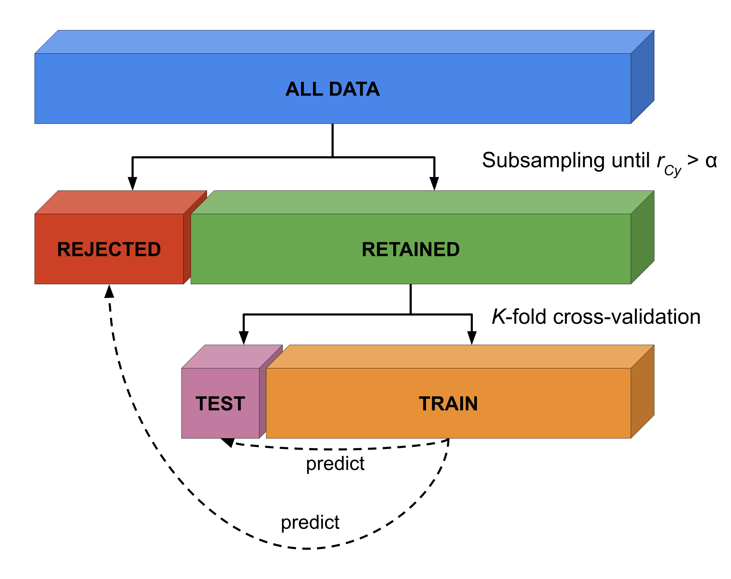
Figure 3.3: Visualization of method to evaluate whether counterbalancing yields unbiased cross-validated model performance estimates.

3.2.4.3 Analysis of negative bias after WDCR

As also detailed below, WDCR can lead to significantly below chance accuracy. To investigate the cause of this below chance performance (and to demonstrate that CVCR does not lead to such results), we performed two follow-up simulations. The first follow-up simulation shows that the occurrence of below chance accuracy depends on the distribution of feature-target correlations ($r_{yX}$; see for a similar argument Jamalabadi et al., 2016), and the second follow-up simulation shows that WDCR artificially narrows this distribution. This artificial narrowing of the distribution is exacerbated both by an increasing number of features ($K$), as well as higher correlations between the target and confound ($r_{Cy}$).

In the first simulation, we simulated random null data (drawn from a standard normal distribution) with 100 samples ($N$) and 200 features ($K$), as well as a binary target feature ($y \in \{0, 1\}$). We then calculated the cross-validated prediction accuracy using the standard pipeline (without univariate feature selection) described in the Decoding pipeline section; we iterate this process 500 times. Then, we show that the variance of the cross-validated accuracy is accurately predicted by the standard deviation (i.e., “width”) of the distribution of correlations between the features and the target ($r_{yX_{j}}$ with $j = 1 \dots K$), which we will denote by $sd(r_{yX})$. Importantly, we show that below chance accuracy likely occurs when the standard deviation of the feature-target correlation distribution is lower than the standard deviation of the sampling distribution of the Pearson correlation coefficient parameterized with the same number of samples ($N = 200$) and the same effect size (i.e., $\rho = 0$, because we simulated random null data). The sampling distribution of the Pearson correlation coefficient is described by Kendall & Stuart (1973). When $\rho = 0$ (as in our simulations), the equation is as follows:

\[\begin{equation} f(r; N) = (1 -r^2)^{\frac{N-4}{2}}[\mathcal{B}](\frac{1}{2}, \frac{N-2}{2})^{-1} \end{equation}\]

where $\mathcal{B}(a, b)$ represents the Beta-function.

Then, in a second simulation, we similarly simulated null data as in the previous simulation, but now we also generate a continuous confound ($C$) with a varying correlation with the target ($r_{Cy} \in \{0.0, 0.1, 0.2, \dots, 1.0\}$). Before subjecting the data to the decoding pipeline, we regressed out the confound from the data (i.e., WDCR). We did this for different numbers of features ($K \in \{1, 5, 10, 50, 100, 500, 1000\}$). Then, we applied CVCR on the simulated data as well for comparison.

3.3 Results

3.3.1 Influence of brain size

Before evaluating the different methods for confound control, we determined whether brain size is truly a confound given our proposed definition (“a variable that is not of primary interest, correlates with the target, and is encoded in the neuroimaging data”). We evaluated the relationship between the target and the confound in two ways. First, we calculated the (point-biserial) correlation between gender and brain size, which was significant for both the estimation based on white matter, $r(216) = .645, p < 0.001$, and the estimation based on grey matter, $r(216) = .588, p < 0.001$, corroborating the findings by Smith & Nichols (2018). Second, as recommended by Görgen et al. (2017), who argue that the potential influence of confounds can be discovered by running a classification analysis using the confound as the (single) feature predicting the target, we ran our decoding pipeline (without univariate feature selection) using brain size as a single feature to predict gender. This analysis yielded a mean classification performance ($F_{1}$ score) of 0.78 (SD = .10) when using brain size estimated from white matter and 0.81 (SD = .09) when using brain size estimated from gray matter, which are both significant with $p < 0.001$ (see Figure 3.4A).

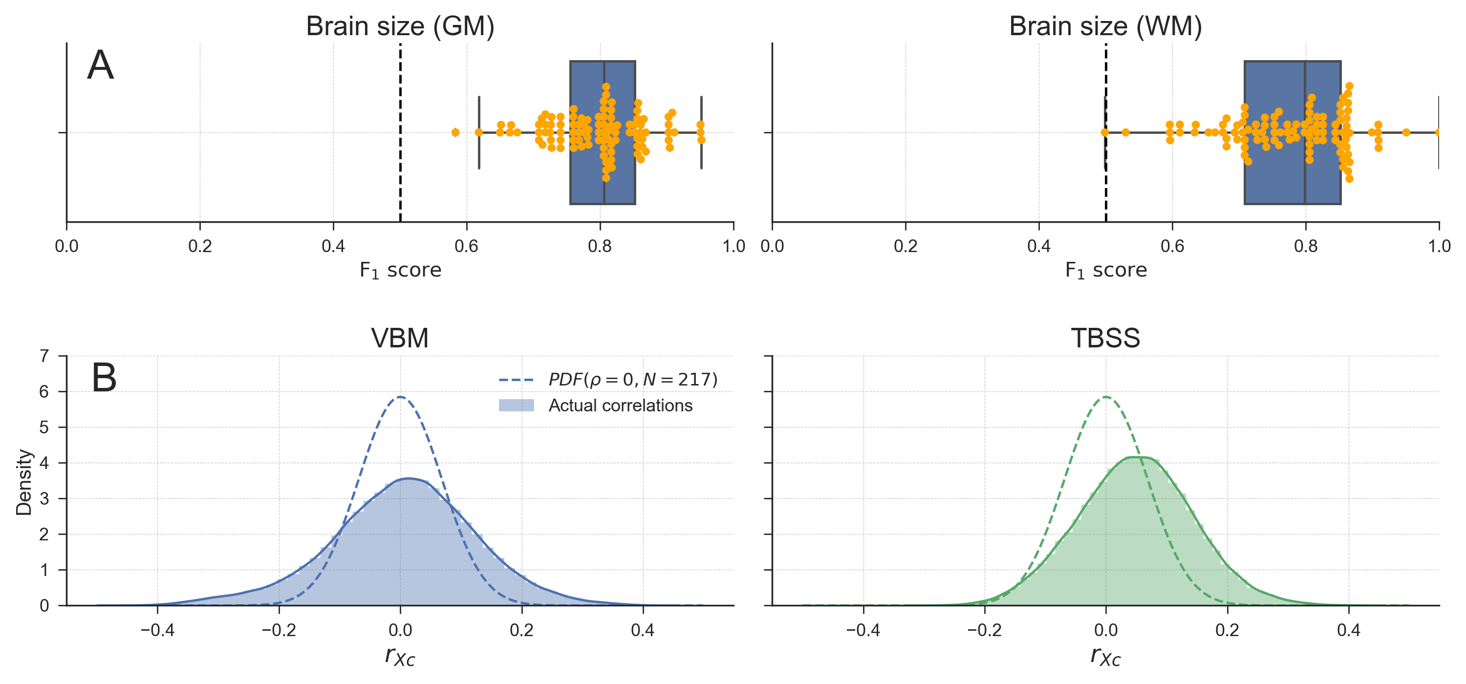
$A) Model performance when using brain size to predict gender for both brain-size estimated from grey matter (left) and from white matter (right). Points in yellow depict individual $F_{1}$ scores per fold in the 10-fold cross-validation scheme. Whiskers of the box plot are 1.5x the interquartile range. B) Distributions of observed correlations between brain size and voxels ($r_{XC}$), overlayed with the analytic sampling distribution of correlation coefficients when $\rho = 0$ and $N = 217$, for both the VBM data (left) and TBSS data (right). Density estimates are obtained by kernel density estimation with a Gaussian kernel and Scott’s rule (Scott, 1979) for bandwidth selection.$

Figure 3.4: A) Model performance when using brain size to predict gender for both brain-size estimated from grey matter (left) and from white matter (right). Points in yellow depict individual $F_{1}$ scores per fold in the 10-fold cross-validation scheme. Whiskers of the box plot are 1.5x the interquartile range. B) Distributions of observed correlations between brain size and voxels ($r_{XC}$), overlayed with the analytic sampling distribution of correlation coefficients when $\rho = 0$ and $N = 217$, for both the VBM data (left) and TBSS data (right). Density estimates are obtained by kernel density estimation with a Gaussian kernel and Scott’s rule (Scott, 1979) for bandwidth selection.

To estimate whether brain size is encoded in the neuroimaging data, we compared the distribution of bivariate correlation coefficients (of each voxel with brain size) with the sampling distribution of correlation coefficients when $\rho = 0$ and $N = 217$ (see section Analysis of negative bias after WDCR for details). Under the null hypothesis that there are no correlations between brain size and voxel intensities, each individual correlation coefficient between a voxel and the confound can be regarded as an independent sample with $N = 217$ (ignoring correlations between voxels for simplicity). Because $K$ is very large for both the VBM and TBSS data, the empirical distribution of correlation coefficients should, under the null hypothesis, approach the analytic distribution of correlation coefficients parametrized by $\rho = 0$ and $N = 217$. Contrarily, the density plots in Fig. 3.4B clearly show that the observed correlation coefficients distribution does not follow the sampling distribution (with both an increase in variance and a shift of the mode). This indicates that at least some of the correlation coefficients between voxel intensities and brain size are extremely unlikely under the null hypothesis. Note that this interpretation is contingent on the assumption that the relation between brain size and VBM/TBSS data is linear. In the Supplementary Materials and Results (Supplementary Figures B.7-B.9), we provide some evidence for the validity of this assumption.

3.3.2 Baseline model: no confound control

In our baseline model on the empirical data, for different numbers of voxels, we predicted gender from structural MRI data (VBM and TBSS) without controlling for brain size (see Figure 3.5). The results show significant above chance performance of the MVPA pipeline based on both the VBM data and the TBSS data. All performance scores averaged across folds were significant ($p < 0.001$).

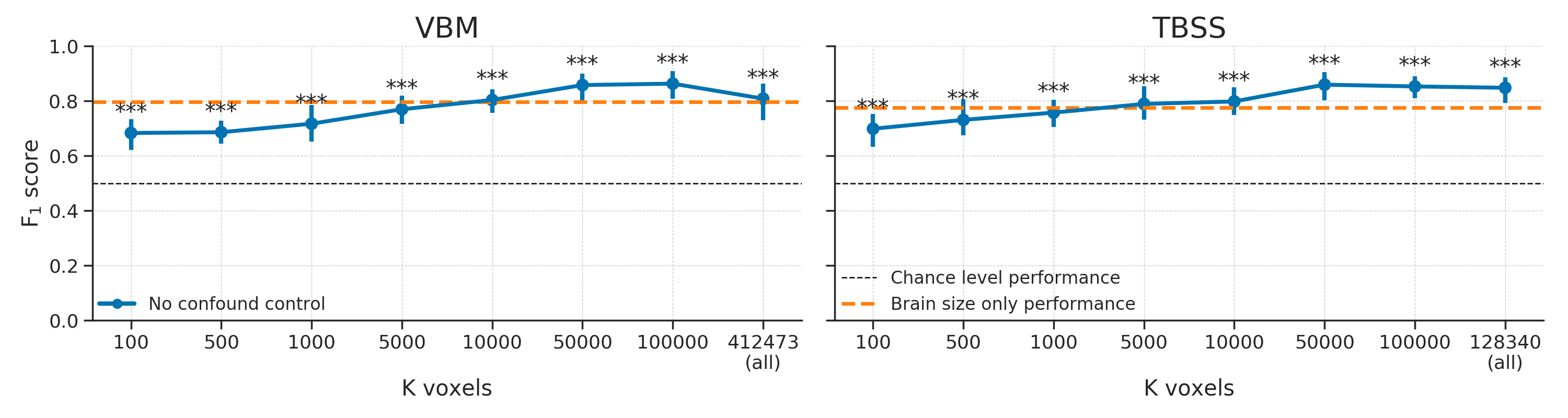
$Baseline scores using the VBM (left) and TBSS (right) data without any confound control. Scores reflect the average $F_{1}$ score across 10 folds; error bars reflect 95% confidence intervals. The dashed black line reflect theoretical chance-level performance and the dashed orange line reflects the average model performance when only brain size is used as a predictor for reference; Asterisks indicates significant performance above chance: *** = $p < 0.001$, ** = $p < 0.01$, * = $p < 0.05$.$

Figure 3.5: Baseline scores using the VBM (left) and TBSS (right) data without any confound control. Scores reflect the average $F_{1}$ score across 10 folds; error bars reflect 95% confidence intervals. The dashed black line reflect theoretical chance-level performance and the dashed orange line reflects the average model performance when only brain size is used as a predictor for reference; Asterisks indicates significant performance above chance: *** = $p < 0.001$, ** = $p < 0.01$, * = $p < 0.05$.

These above chance performance estimates replicate previous studies on gender decoding using structural MRI data (Del Giudice et al., 2016; Rosenblatt, 2016; Sepehrband et al., 2018) and will serve as a baseline estimate of model performance to which the confound control methods will be compared.

In the next three subsections, we will report the results from the three discussed methods to control for confounds: post hoc counterbalancing, whole-dataset confound regression (WDCR), and cross-validated confound regression (CVCR).

3.3.3 Post hoc counterbalancing

3.3.3.1 Empirical results

In order to decorrelate brain size and gender (i.e., $r_{Cy} > 0.1$), our subsampling algorithm selected 117 samples in the VBM data (i.e., a sample size reduction of 46.1%) and 131 samples in the TBSS data (i.e., a reduction of 39.6%). The model performance for different values of (number of voxels) are shown in Figure 3.6. Contrary to our expectations, the predictive accuracy of our decoding pipeline after counterbalancing was similar to baseline performance. This is particularly surprising in light of the large reductions in sample size, which results in a substantial loss in power, which in turn is expected to lead to lower model performance.

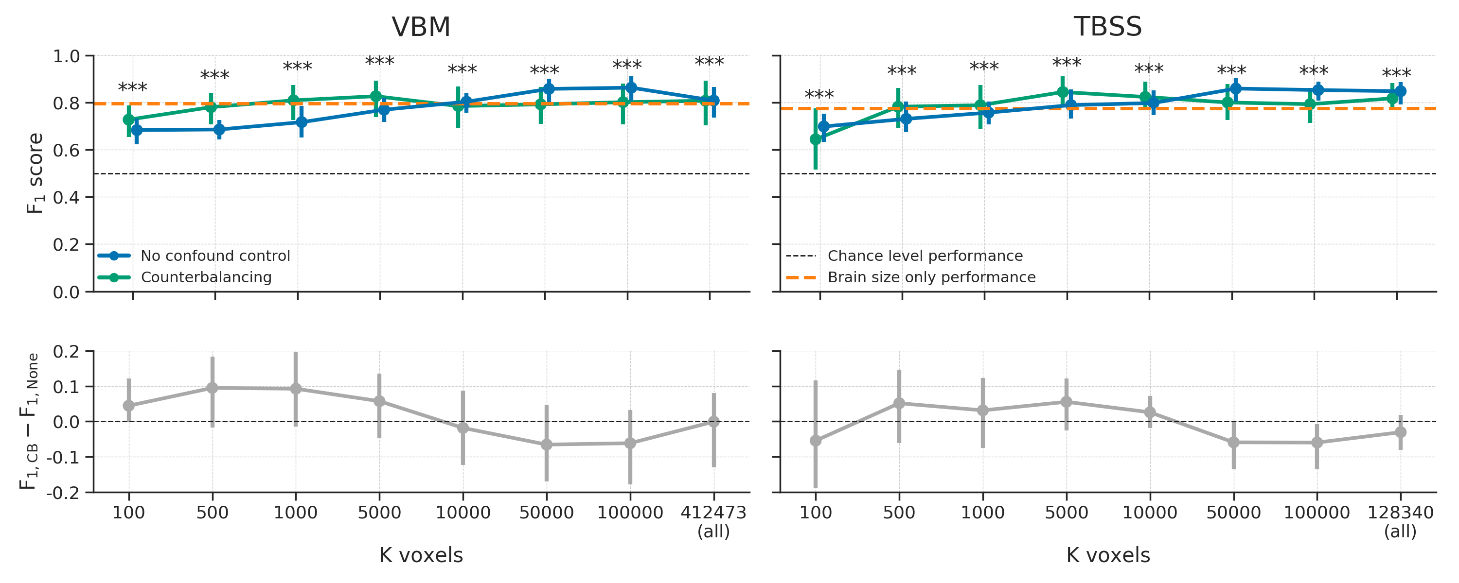
$Model performance after counterbalancing (green) versus the baseline performance (blue) for both the VBM (left) and TBSS (right) data (upper row) and the difference in performance between the methods (lower row). Performance reflects the average (difference) $F_{1}$ score across 10 folds; error bars reflect 95% confidence intervals. The dashed black line reflect theoretical chance-level performance (0.5) and the dashed orange line reflects the average model performance when only brain size is used as a predictor. Asterisks indicates significant performance above chance: *** = $p < 0.001$, ** = $p < 0.01$, * = $p < 0.05$.$

Figure 3.6: Model performance after counterbalancing (green) versus the baseline performance (blue) for both the VBM (left) and TBSS (right) data (upper row) and the difference in performance between the methods (lower row). Performance reflects the average (difference) $F_{1}$ score across 10 folds; error bars reflect 95% confidence intervals. The dashed black line reflect theoretical chance-level performance (0.5) and the dashed orange line reflects the average model performance when only brain size is used as a predictor. Asterisks indicates significant performance above chance: *** = $p < 0.001$, ** = $p < 0.01$, * = $p < 0.05$.

One could argue that the lack of expected decrease in model performance after counterbalancing can be explained by the possibility that the subsampling and counterbalancing procedure just leads to the selection of different features during univariate feature selection compared to the baseline model. In other words, the increase in model performance may be caused by the feature selection function, which selects “better” voxels (i.e., containing more “robust” signal), resulting in similar model performance in spite of the reduction in sample size. However, this does not explain the similar scores for counterbalancing and the baseline model when using all voxels (the data points at ‘$K\ \mathrm{voxels} = \dots \mathrm{(all)}$’ in Figure 3.6). Another possibility for the relative increase in model performance based on the counterbalanced data versus the baseline model is that counterbalancing increased the amount of signal in the data. Indeed, counterbalancing appeared to increase the (absolute) correlations between the data and the target ($r_{yX}$), which is visualized in Figure 3.7, suggesting an increase in signal.

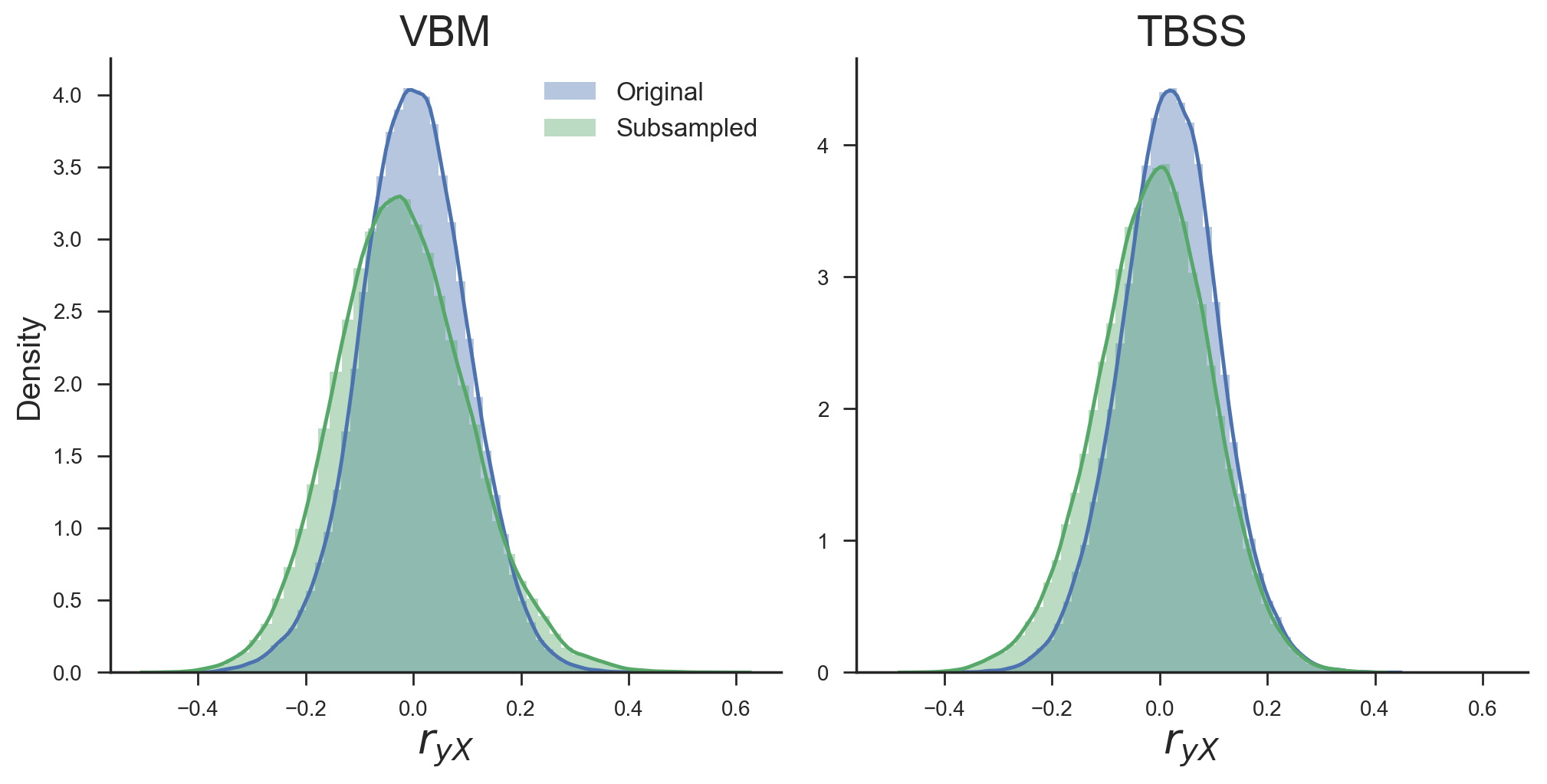
Density plots of the correlations between the target and voxels across all voxels before (blue) and after (green) subsampling for both the VBM and TBSS data. Density estimates are obtained by kernel density estimation with a Gaussian kernel and Scott’s rule (Scott, 1979) for bandwidth selection.

Figure 3.7: Density plots of the correlations between the target and voxels across all voxels before (blue) and after (green) subsampling for both the VBM and TBSS data. Density estimates are obtained by kernel density estimation with a Gaussian kernel and Scott’s rule (Scott, 1979) for bandwidth selection.

This apparent increase in the correlations between the target and neuroimaging data goes against the intuition that removing the influence of a confound that is highly correlated with the target will reduce decoding performance. To further investigate this, we replicated this effect of post hoc counterbalancing on simulated data, as described in the next section (Efficacy analyses), and additionally investigated the cause of the negative bias observed after WDCR using a separate set of simulations.

3.3.3.2 Efficacy analysis

To evaluate the efficacy of the three confound control methods, we simulated data in which we varied the strength of confound $R^2$ and signal $R^2$, after which we applied the three confound control methods to the data. The results of this analysis show that counterbalancing maintains chance-level model performance when there is almost no signal in the data (i.e., signal $R^2 = 0.004$; Figure 3.8, left graph, green line). However, when there is some signal (i.e., signal $R^2 = 0.1$; Fig. 8, right graph), we observed that counterbalancing yields similar or even higher scores than the baseline model, replicating the effects observed in the empirical analyses.

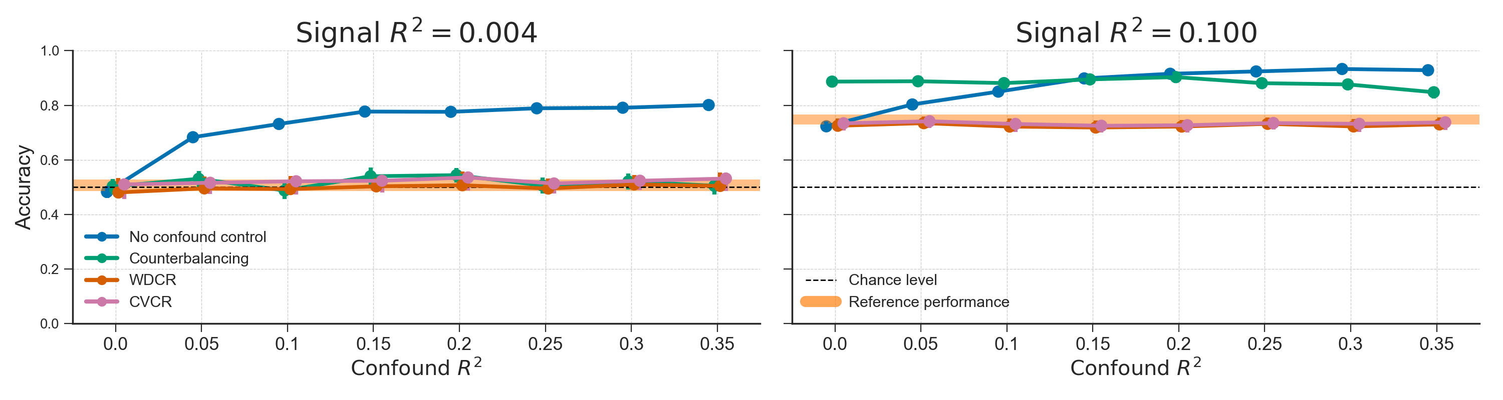
$Results from the different confound control methods on simulated data without any experimental effect (signal $R^2 = 0.004$; left graph) and with some experimental effect (signal $R^2 = 0.1$; right graph) for different values of confound $R^2$. The orange line represents the average performance (±1 SD) when confound $R^2 = 0$, which serves as a “reference performance” for when there is no confounded signal in the data. For both graphs, the correlation between the target and the confound, $r_{yC}$, is fixed at 0.65. The results from the WDCR and CVCR methods are explained later.$

Figure 3.8: Results from the different confound control methods on simulated data without any experimental effect (signal $R^2 = 0.004$; left graph) and with some experimental effect (signal $R^2 = 0.1$; right graph) for different values of confound $R^2$. The orange line represents the average performance (±1 SD) when confound $R^2 = 0$, which serves as a “reference performance” for when there is no confounded signal in the data. For both graphs, the correlation between the target and the confound, $r_{yC}$, is fixed at 0.65. The results from the WDCR and CVCR methods are explained later.

As is apparent from Figure 3.8 (right panel), when there is some signal, the counterbalanced data seem to yield better performance than the baseline model only for relatively low confound $R^2$ values (confound $R^2 < 0.15$). As suggested by our findings in the empirical data (see Figure 3.7), we hypothesized that the observed improvement in model performance after counterbalancing was caused by the increase in correlations between the target and features in the neuroimaging data. In support of this hypothesis, Figure 3.9 illustrates the relations between the strength of the confound (confound $R^2$, color coded), the increase in correlations after post hoc counterbalancing ($\delta r_{yX} = r_{yX}^{\mathrm{after}} - r_{yX}^{\mathrm{after}}$; x-axis) for each confound $R^2$, and the resulting difference in model performance ($\mathrm{ACC}_{\mathrm{CB}} - \mathrm{ACC}_{\mathrm{baseline}}$; y-axis). The figure shows that the increase or decrease in accuracy after counterbalancing (compared to baseline) depends on $\delta r_{yX}$ ($r(79) = .922$, $p < 0.001$), which in turn depends on confound $R^2$ ($r(79) = -0.987$, $p < 0.001$). To reiterate, these differences in model performance are only due to the post hoc counterbalancing procedure and not due to varying signal in the simulated data. The effect of post hoc counterbalancing on model performance thus seems to depend on the strength of the confound.

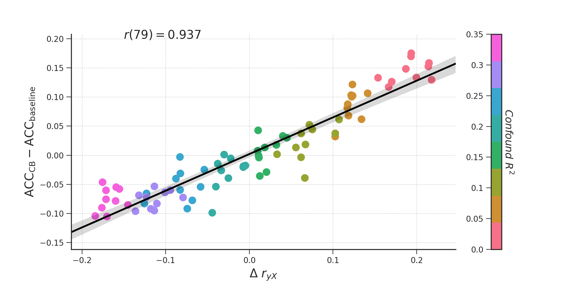
$The relationship between the increase in correlations between target and data ($r_{yX}$) after subsampling, confound $R^2$, difference in model performance (here: accuracy) between the counterbalance model and baseline model ($\mathrm{ACC}_{\mathrm{CB}} - \mathrm{ACC}_{\mathrm{baseline}}$).$

Figure 3.9: The relationship between the increase in correlations between target and data ($r_{yX}$) after subsampling, confound $R^2$, difference in model performance (here: accuracy) between the counterbalance model and baseline model ($\mathrm{ACC}_{\mathrm{CB}} - \mathrm{ACC}_{\mathrm{baseline}}$).

While this relationship in Figure 3.9 might be statistically interesting, it does not explain why post hoc counterbalancing tends to increase the correlations between neuroimaging data and target, and even outperforms the baseline model when confound $R^2$ is low and some signal is present. More importantly, it does not tell us whether the post hoc counterbalancing procedure uncovers signal that is truly related to the target — in which case the procedure suppresses noise — or inflates performance estimates and thereby introduces positive bias. Therefore, in the next section, we report and discuss results from a follow-up simulation that intuitively shows why post hoc counterbalancing leads to an increase in performance, and furthermore shows that this increase is in fact a positive bias.

3.3.3.3 Analysis of positive bias after post hoc counterbalancing

With this follow-up analysis, we aimed to visualize the scenario in which post hoc counterbalancing leads to a clearly better performance than model performance without confound control. As such, we generated 1000 data sets using a covariance matrix that we knew leads to a large difference between the baseline model and model performance after counterbalancing (i.e., data with a low confound $R^2$). From these 1000 datasets, we selected the dataset that yielded the largest difference for our visualization (see the Analysis of positive bias after post hoc counterbalancing section in the Methods for details).

The data that yielded the largest difference (i.e., a performance increase from 0.613 to 0.804, a 31% increase) are visualized in Figure 3.10. Each sample’s confound value ($C$) is plotted against its feature value ($X$), both before subsampling (upper scatter plot) and after subsampling (lower scatter plot). From visual inspection, it appears that the samples rejected by the subsampling procedure (i.e., the samples with the white border) have relatively large absolute values of the confound variable, which tend to lie close to or on the “wrong” side of the classification boundary (i.e., the dashed black line) in this specific configuration of the data. In other words, subsampling seems to reject samples that are harder to classify or would be incorrectly classified based on the data (here, the single feature of $X$). The density plots in Figure 3.10 show the same effect in a different way: while the difference in the modes of the distributions of the confound ($C$) between classes is reduced after subsampling (i.e., the density plots parallel to the y-axis), the difference in the modes of the distributions of the data ($X$) between classes is actually increased after subsampling (i.e., the density plots parallel to the x-axis).

$Both scatterplots visualize the relationship between the data ($X$ with $K=1$, on the x-axis), the confound ($C$, on the y-axis) and the target ($y$). Dots with a white border in the upper scatterplot indicate samples that are rejected in the subsampling process; the lower scatterplot visualizes the data without these rejected samples. The dashed black lines in the scatterplot represent the decision boundary of the SVM classifier; the color of the background shows how samples in that area are classified (a blue background means a prediction of $y = 0$ and a green background means a prediction of $y = 1$). The density plots parallel to the y-axis depict the distribution of the confound ($C$) for the samples in which $y = 0$ (blue) and in which $y = 1$ (green). The density plots parallel to x-axis depict the distribution of the data ($X$) for the samples in which $y = 0$ (blue) and in which $y = 1$ (green). Density estimates are obtained by kernel density estimation with a Gaussian kernel and Scott’s rule (Scott, 1979) for bandwidth selection.$

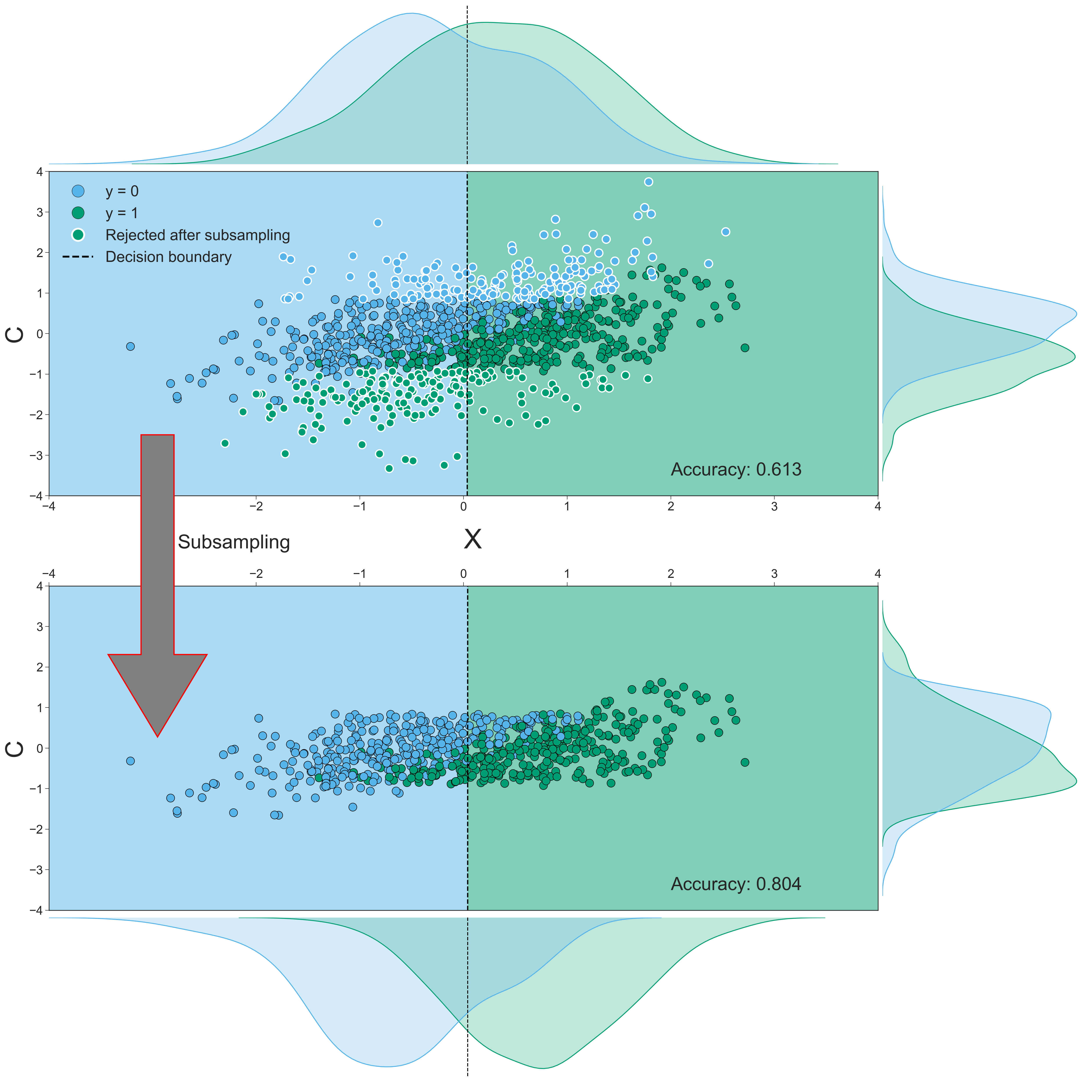
Figure 3.10: Both scatterplots visualize the relationship between the data ($X$ with $K=1$, on the x-axis), the confound ($C$, on the y-axis) and the target ($y$). Dots with a white border in the upper scatterplot indicate samples that are rejected in the subsampling process; the lower scatterplot visualizes the data without these rejected samples. The dashed black lines in the scatterplot represent the decision boundary of the SVM classifier; the color of the background shows how samples in that area are classified (a blue background means a prediction of $y = 0$ and a green background means a prediction of $y = 1$). The density plots parallel to the y-axis depict the distribution of the confound ($C$) for the samples in which $y = 0$ (blue) and in which $y = 1$ (green). The density plots parallel to x-axis depict the distribution of the data ($X$) for the samples in which $y = 0$ (blue) and in which $y = 1$ (green). Density estimates are obtained by kernel density estimation with a Gaussian kernel and Scott’s rule (Scott, 1979) for bandwidth selection.

We quantified this effect of subsampling by comparing the signed distance from the decision boundary (i.e., the dashed line in the upper scatter plot) between the retained samples and the rejected (subsampled) samples, in which a larger distance from the decision boundary reflects a higher confidence of the classifier’s prediction (see Figure 3.3 for a visualization of this method). Indeed, we found that samples that are removed by subsampling lie significantly closer to (or on the “wrong” side of) the decision boundary (M = -.358, SD = .619) than samples that are retained after subsampling (M = .506, SD = .580), as indicated by an independent samples t-test, $t(998) = 22.32$, $p < 0.001$. Also (which follows from the previous observation), samples that would have been removed by subsampling are more often classified incorrectly (75% incorrect) than the samples that would have been retained by subsampling (20% incorrect), as indicated by a chi-squared test, $\chi^{2} = 270.29$, $p < 0.001$.

To show that the same effect (i.e., removing samples that tend to be hard to classify or would be wrongly classified) occurred in the empirical data after counterbalancing as well, we applied the same analysis of comparing model performance and distance to boundary between the retained and rejected samples to the empirical data. Indeed, across all different numbers of voxels ($K$), the retained samples were significantly more often classified correctly (Figure 3.11A) and had a significantly larger distance to the classification boundary (Figure 3.11B) than the rejected samples. This demonstrates that the same effect of post hoc counterbalancing, as shown in the simulated data, likely underlies the increase in model performance of the counterbalanced data relative to the baseline model in the empirical data.

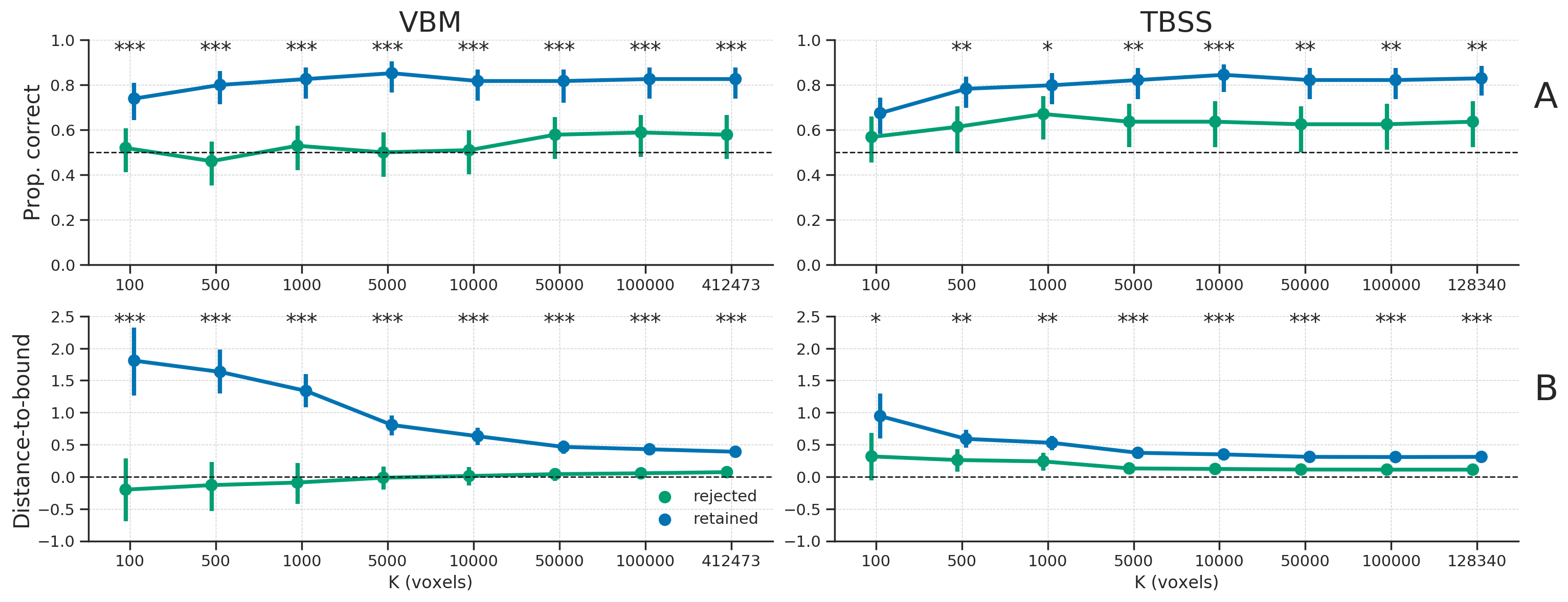
$A) The proportion of samples classified correctly, separately for the “retained” samples (blue line) and “rejected” samples (green line); the dashed line represents chance level (0.5). B) The average distance to the classification boundary for the retained and rejected samples; the dashed line represents the decision boundary, with values below the line representing samples on the “wrong” side of the boundary (and vice versa). Asterisks indicates a significant difference between the retained and rejected samples: *** = $p < 0.001$, ** = $p < 0.01$, * = $p < 0.05$.$

Figure 3.11: A) The proportion of samples classified correctly, separately for the “retained” samples (blue line) and “rejected” samples (green line); the dashed line represents chance level (0.5). B) The average distance to the classification boundary for the retained and rejected samples; the dashed line represents the decision boundary, with values below the line representing samples on the “wrong” side of the boundary (and vice versa). Asterisks indicates a significant difference between the retained and rejected samples: *** = $p < 0.001$, ** = $p < 0.01$, * = $p < 0.05$.

One can wonder how much the occurrence of these observed biases in post hoc counterbalancing depends on the specific method of subsampling used. Random subsampling led to qualitatively similar results as targeted subsampling (cf. Supplementary Figures B.13 and B.14 with random subsampling). Instead, the bias is introduced through features that weakly correlate with the target in the whole sample, but strongly in subsamples where there is no correlation between target and the confound (features which, as our results show, exist in the neuroimaging data). That is, the bias is an indirect result of decorrelating target and confound in the sample, which is an essential step in post hoc counterbalancing (in fact, it is the goal of counterbalancing). For this reason, we consider it unlikely (but not impossible) that there exists a way to subsample data without introducing biases.

In summary, removing a subset of observations to correct for the influence of a confound can induce substantial bias by removing samples that are harder to classify using the available data. The bias itself can be subtle (e.g., in our empirical results, the predictive performance falls in a realistic range of predictive performances), and could remain undetected when present. Therefore, we believe that post hoc counterbalancing by subsampling the data is an inappropriate method to control for confounds.

3.3.4 Whole-dataset confound regression (WDCR)

3.3.4.1 Empirical results

In addition to post hoc counterbalancing, we evaluated the efficacy of “whole-dataset confound regression” (WDCR), i.e. regressing out the confound from each feature separately using all samples from the dataset to control for confounds. Compared to the baseline model, WDCR yielded a strong decrease in performance, even dropping (significantly) below chance for all TBSS analyses and a subset of the VBM analyses (see Figure 3.12).

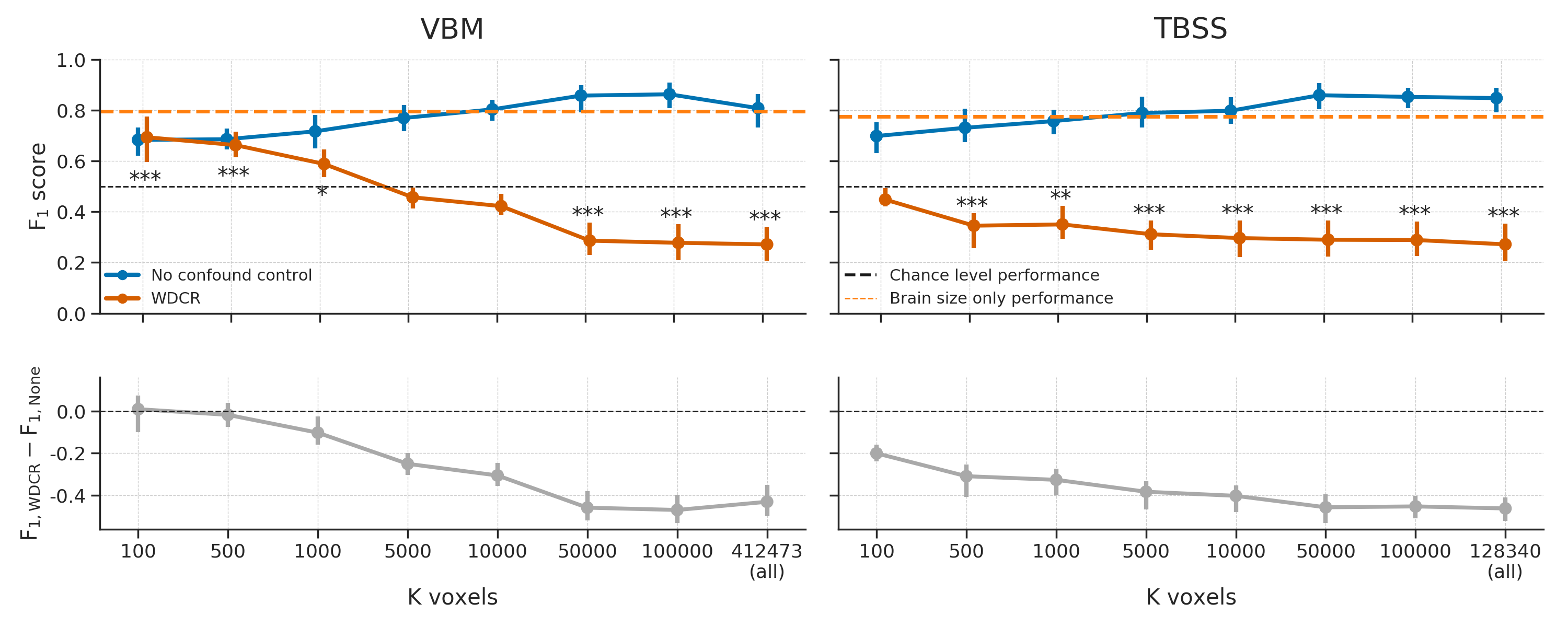
$Model performance after WDCR (orange) versus the baseline performance (blue) for both the VBM (left) and TBSS (right) data. Performance reflects the average $F_{1}$ score across 10 folds; error bars reflect 95% confidence intervals. The dashed black line reflect theoretical chance-level performance (0.5) and the dashed orange line reflects the average model performance when only brain size is used as a predictor. Asterisks indicates performance of the WDCR model that is significantly above or below chance: *** = $p < 0.001$, ** = $p < 0.01$, * = $p < 0.05$.$

Figure 3.12: Model performance after WDCR (orange) versus the baseline performance (blue) for both the VBM (left) and TBSS (right) data. Performance reflects the average $F_{1}$ score across 10 folds; error bars reflect 95% confidence intervals. The dashed black line reflect theoretical chance-level performance (0.5) and the dashed orange line reflects the average model performance when only brain size is used as a predictor. Asterisks indicates performance of the WDCR model that is significantly above or below chance: *** = $p < 0.001$, ** = $p < 0.01$, * = $p < 0.05$.

This strong (and implausible) reduction in model performance after WDCR is investigated in more detail in the next two sections on the results from the simulations.

3.3.4.2 Efficacy analysis

The results from the analyses investigating the efficacy of the confound control methods (see Figure 3.8) show that WDCR accurately corrects for the confound in both in data without signal (i.e., when signal $R^2 = 0.004$) and in data with some signal (i.e., when signal $R^2 = 0.1$), as evident from the fact that the performance after WDCR is similar to the reference performance. This result (i.e., plausible performance after confound control) stands in contrast to the results from the empirical analyses, which is why we ran a follow-up analysis on simulated data to investigate this specific issue.

3.3.4.3 Analysis of negative bias after WDCR

Inspired by the work of Jamalabadi et al. (2016) on below chance accuracy in decoding analyses, we ran several follow-up analyses to get insight into why WDCR leads to below chance model performance. As Jamalabadi et al. show, below chance model performance occurs when the data contain little signal. In our first follow-up simulation, we sought to refine the explanation of the cause of below chance model performance by linking it to the observed standard deviation of the empirical distribution of correlations between the data ($X$) and the target ($y$). To do so, we simulated random data ($X$) and a binary target ($y \in \{0, 1\}$) and estimated (per fold) the cross-validated classification accuracy using the standard pipeline described in the methods section. We repeated this process 500 times, yielding 500 data sets. The expected average predictive accuracy for each dataset is 0.5, but this varies randomly across folds and iterations. We hypothesized that this variance can be explained by the standard deviation (“width”) of the initial feature-target correlation distribution, sd($r_{Xy}$): narrower distributions may yield relatively lower cross-validated classification accuracy than relatively wider feature-target correlation distributions. Indeed, we find that the initial standard deviation of this distribution is significantly correlated with the cross-validated accuracy, $r(499) = 0.73$, $p < 0.001$ (Figure 3.13A). Importantly, we find that this relationship holds for different values of $N$ (see Supplementary Figure B.15, for different sizes of the test set (see Supplementary Figure B.16), and for different sizes of $K$ (see Supplementary Figure B.17).

$A) The relationship between the standard deviation of the distribution of feature-target correlations, sd($r_{yX}$), and accuracy across iterations of cross-validated classification analyses of null data. The vertical dashed line represents the standard deviation from the sampling distribution parameterized with $\rho = 0$ and $N = 100$ (i.e., the same parameters used to generate the null data); the horizontal dashed line represents the expected accuracy for data with this standard deviation based on the regression line estimated from the data across simulations (see Supplementary Figure B.15 for the same plot with different values for $N$). B) The relationship between the proportion of features of which the sign of their correlation with the target ($r_{Xy}$) “flips” between the train-set and the test-set and accuracy. The vertical dashed line represents a proportion of 0.5., i.e., 50% of the features flip their correlation sign, which corresponds approximately with an accuracy of 0.5. C) The relationship between the weighted difference between feature-target correlations in the train and test set (see equation (3.3)) and accuracy.$

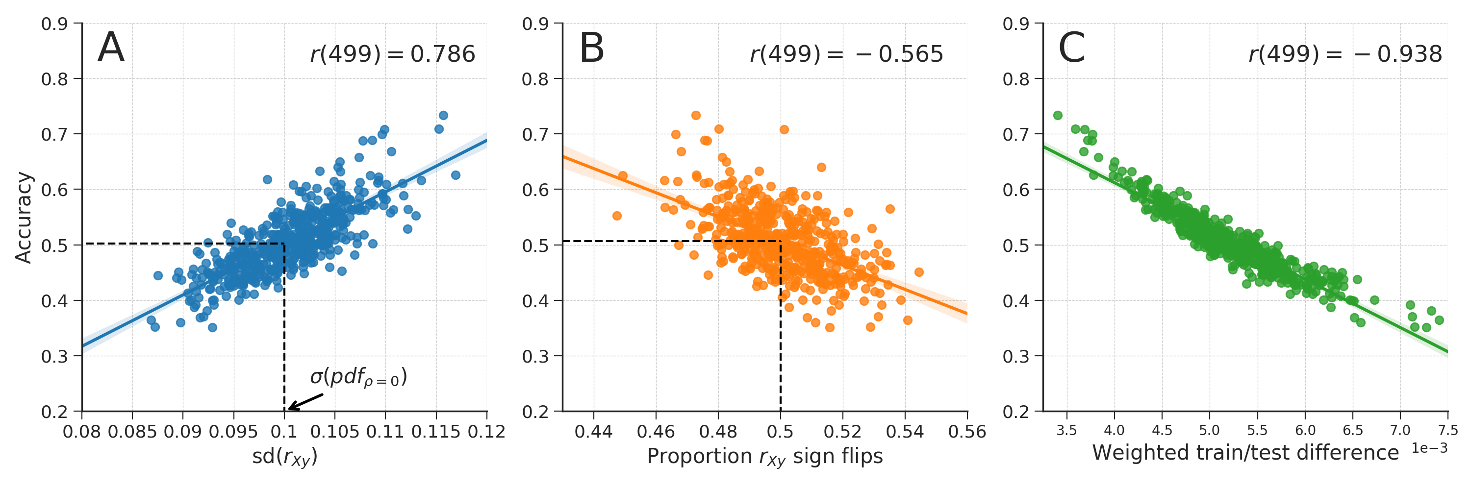
Figure 3.13: A) The relationship between the standard deviation of the distribution of feature-target correlations, sd($r_{yX}$), and accuracy across iterations of cross-validated classification analyses of null data. The vertical dashed line represents the standard deviation from the sampling distribution parameterized with $\rho = 0$ and $N = 100$ (i.e., the same parameters used to generate the null data); the horizontal dashed line represents the expected accuracy for data with this standard deviation based on the regression line estimated from the data across simulations (see Supplementary Figure B.15 for the same plot with different values for $N$). B) The relationship between the proportion of features of which the sign of their correlation with the target ($r_{Xy}$) “flips” between the train-set and the test-set and accuracy. The vertical dashed line represents a proportion of 0.5., i.e., 50% of the features flip their correlation sign, which corresponds approximately with an accuracy of 0.5. C) The relationship between the weighted difference between feature-target correlations in the train and test set (see equation (3.3)) and accuracy.

This observation, then, begs the question: why do narrower-than-chance correlation distributions lead to below chance accuracy? One potential explanation of below chance accuracy is that the classifier may learn a particular (linear) relationship between features and the target in the train set (e.g., $r_{Xy} = 0.05$), while the sign of this relationship is “flipped” in the test set (e.g., $r_{Xy} = -0.03$; see Jamalabadi et al., 2016), which is known in the machine learning literature as “dataset shift” (Quionero-Candela et al., 2009). This situation would lead classifiers to predict the exact opposite classes for samples in the test set, leading to below chance accuracy. In the results of our simulated data, the standard deviation of the feature-target distribution was indeed significantly negatively correlated with the proportion of features that flipped the sign of their correlation between the train set and test set, $r(499) = -.687$, $p < 0.001$. This means that a higher density of feature-target correlations around 0 (i.e., a narrower width of the corresponding distribution) leads to more “sign flips”. This phenomenon of “sign flipping” has been reported before in the context of (a priori) counterbalancing of categorical variables ($X$) with respect to the target ($y$), where it was observed that complete counterbalancing led to consistent “sign flipping” and consequently 0% accuracy (Görgen et al., 2017). Similarly, we found that the proportion of features that flip sign was significantly negatively correlated with accuracy, $r = -.565$, $p < 0.001$, indicating that larger proportions of features that flip sign leads to lower accuracy (see Figure 3.13B). Interestingly, at a proportion of 0.5, accuracy is approximately at chance level (0.5; dashed lines in Figure 3.13B).

This relationship between “sign flipping” and accuracy, however, leaves room for improvement in terms of explaining the variance of accuracy scores. Therefore, we sought to further refine our “model” of accuracy by defining dataset shift not by the proportion of sign flips, but by the average difference between the feature-target correlations between the train set and test set. Moreover, because not all features contribute equally strongly to a classifier’s prediction (i.e., they are weighted), we furthermore weighed each feature’s “shift” by the associated classifier weight ($w_{j}$). Formally, we estimated dataset shift ($\hat{ds}$) thus as follows:

\[\begin{equation} \hat{ds} = \frac{1}{K}\sum_{j=1}^{K}(r_{X_{j,\mathrm{train}},y_\mathrm{train}} - r_{X_{j,\mathrm{test}},y_\mathrm{test}})w_{j} \tag{3.3} \end{equation}\]

Indeed, the correlation between this particular operationalization of “dataset shift” and accuracy across simulations was much higher than just the proportion of sign flips, $r(499) = −0.934$ (Figure 3.13B).

Having established the relation between the standard deviation of the initial feature-target correlation distribution and accuracy, we followed up our simulation by investigating specifically the effect of WDCR on the standard deviation of the correlation distribution. We investigated this by simulating data with different strengths of the correlation between the confound and the target ($r_{Cy}$) and the number of features ($K$). From Figure 3.14A, it is clear that, while the expected chance level is 0.5 in all cases, model performance quickly drops below chance for increasing correlations between the target and the confound, as well as for increasing numbers of features; even leading to a model performance of 0% when the confound is perfectly correlated with the target and when using 1000 features. Figure 3.14C shows that, indeed, higher values lead to narrower correlation distributions, which is shown in Figure 3.14D to yield relatively lower accuracy scores.

$A) The effect of WDCR on data varying in the correlation of the confound with the target ($r_{Cy}$; x-axis) and the number of features ($K$; different lines). B) The effect of CVCR on data varying in the correlation of the confound with the target and the number of features. The dashed black line represents chance model performance in subplots A and B. C) The relation between the correlation of the confound with the target ($r_{Cy}$) and the standard deviation of the feature-target correlation distribution, sd($r_{yX}$) for the WDCR data. The dashed black line represents the standard deviation of the correlation distribution predicted by the sampling distribution. D) The relation of the standard deviation of the correlation distribution and accuracy for the WDCR data (only shown for the data when $K = 100$; see Supplementary Figure B.18 for visualizations of this effect for different values of $K$). The data depicted in all panels are null data.$

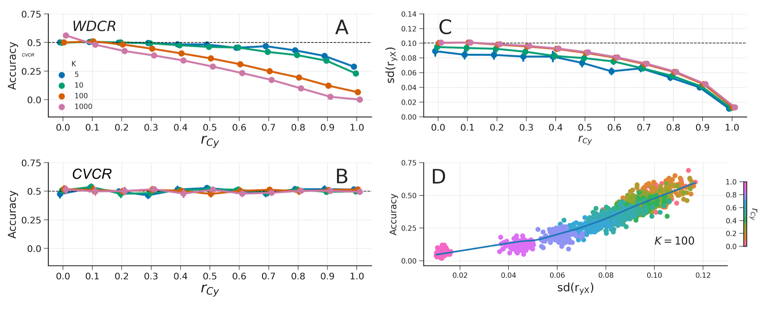
Figure 3.14: A) The effect of WDCR on data varying in the correlation of the confound with the target ($r_{Cy}$; x-axis) and the number of features ($K$; different lines). B) The effect of CVCR on data varying in the correlation of the confound with the target and the number of features. The dashed black line represents chance model performance in subplots A and B. C) The relation between the correlation of the confound with the target ($r_{Cy}$) and the standard deviation of the feature-target correlation distribution, sd($r_{yX}$) for the WDCR data. The dashed black line represents the standard deviation of the correlation distribution predicted by the sampling distribution. D) The relation of the standard deviation of the correlation distribution and accuracy for the WDCR data (only shown for the data when $K = 100$; see Supplementary Figure B.18 for visualizations of this effect for different values of $K$). The data depicted in all panels are null data.

In summary, our simulations show that below chance accuracy is accurately predicted by the standard deviation (i.e., “width”) of the distribution of empirical feature-target correlations and that WDCR reduces this standard deviation, which explains why the empirical analyses yielded below chance model performance (especially for larger numbers of voxels).

3.3.5 Cross-validated confound regression (CVCR)

3.3.5.1 Empirical results

As the results from the empirical analyses and simulations suggest, the use of WDCR is problematic because of the partitioning of the dataset into a separate train set and test set after confound regression. As such, our proposed cross-validated confound regression (CVCR) methods suggests to move the confound regression procedure inside the cross-validation loop, thereby also cross-validating this step. As expected, compared to the baseline model (i.e., no confound control), the results from the empirical analyses using CVCR show reduced (but not below chance) model performance for both VBM and TBSS data, and all different numbers of voxels (see Figure 3.15). Notably, for some numbers of voxels, model performance was not significantly above chance level.

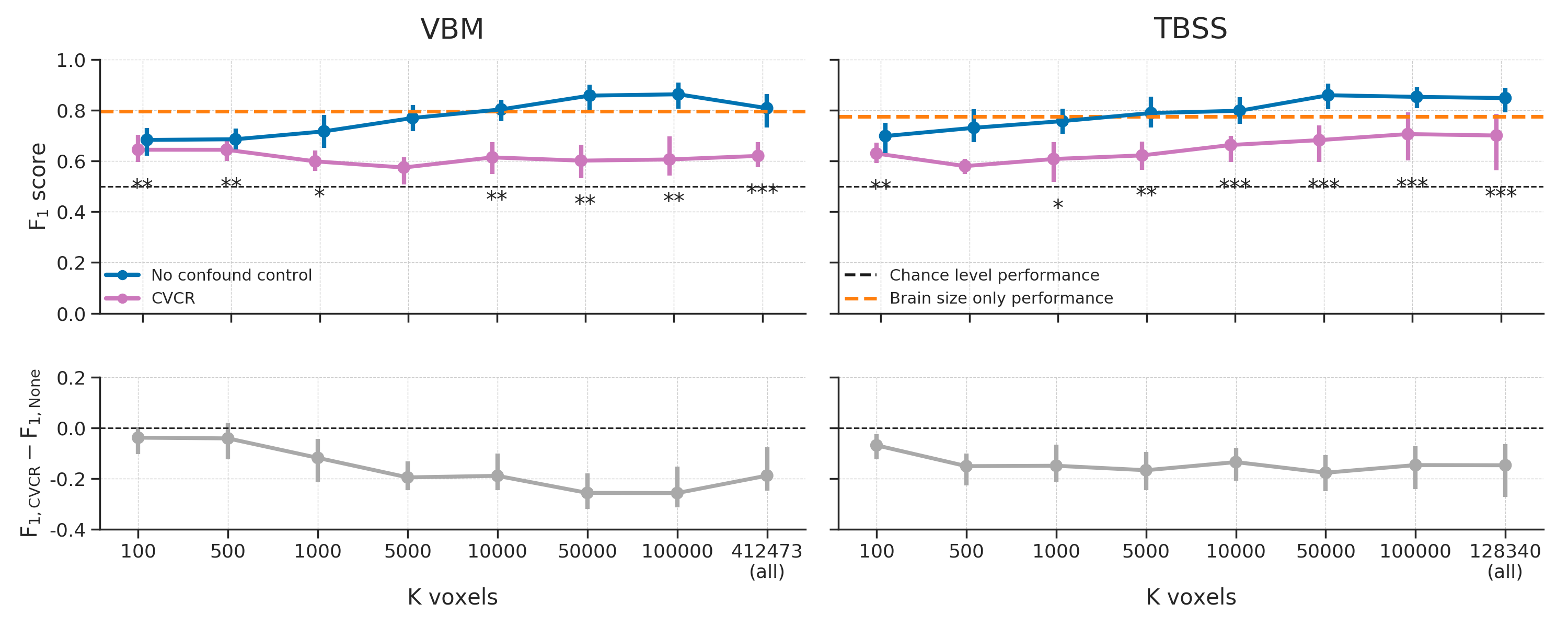
$Model performance after CVCR (pink) versus the baseline performance (blue) for both the VBM (left) and TBSS (right) data. Performance reflects the average $F_{1}$ score across 10 folds; error bars reflect 95% confidence intervals across 1000 bootstrap replications. The dashed black line reflect theoretical chance level performance (0.5) and the dashed orange line reflects the average model performance when only brain size is used as a predictor. Asterisks indicates performance of the CVCR model that is significantly above or below chance: *** = $p < 0.001$, ** = $p < 0.01$, * = $p < 0.05$.$

Figure 3.15: Model performance after CVCR (pink) versus the baseline performance (blue) for both the VBM (left) and TBSS (right) data. Performance reflects the average $F_{1}$ score across 10 folds; error bars reflect 95% confidence intervals across 1000 bootstrap replications. The dashed black line reflect theoretical chance level performance (0.5) and the dashed orange line reflects the average model performance when only brain size is used as a predictor. Asterisks indicates performance of the CVCR model that is significantly above or below chance: *** = $p < 0.001$, ** = $p < 0.01$, * = $p < 0.05$.

We also evaluated whether regressing the confound from the train set only was sufficient to control for confounds, but found that it does not effectively control for confounds when there is no true signal (i.e., there is positive bias), which is visualized in more detail in Supplementary Figure B.10 (cf. Figure 3.8).

3.3.5.2 Efficacy analysis

Similar to WDCR, CVCR yielded plausible and unbiased model performance (see Figure 3.8, pink line). Moreover, when applied to the simulated null data, CVCR yielded model performance scores at chance level across all levels of the confound-target correlation and numbers of features (see Figure 3.14B).

3.3.6 Summary methods for confound control

In this section, we investigated the effects of different method to control confounds (post hoc counterbalancing, WDCR, and CVCR) on empirical MRI data and simulated data (see Figure 3.16 for a summary of the empirical results). Post hoc counterbalancing was, at least using the subsampling method described, clearly unable to effectively control for confounding influences, which is putatively caused by indirect circularity in the analysis process due to subsampling. Confound regression showed an expected drop in model performance (but not below chance level), but only when the confound regression step is properly cross-validated (i.e., the CVCR version).

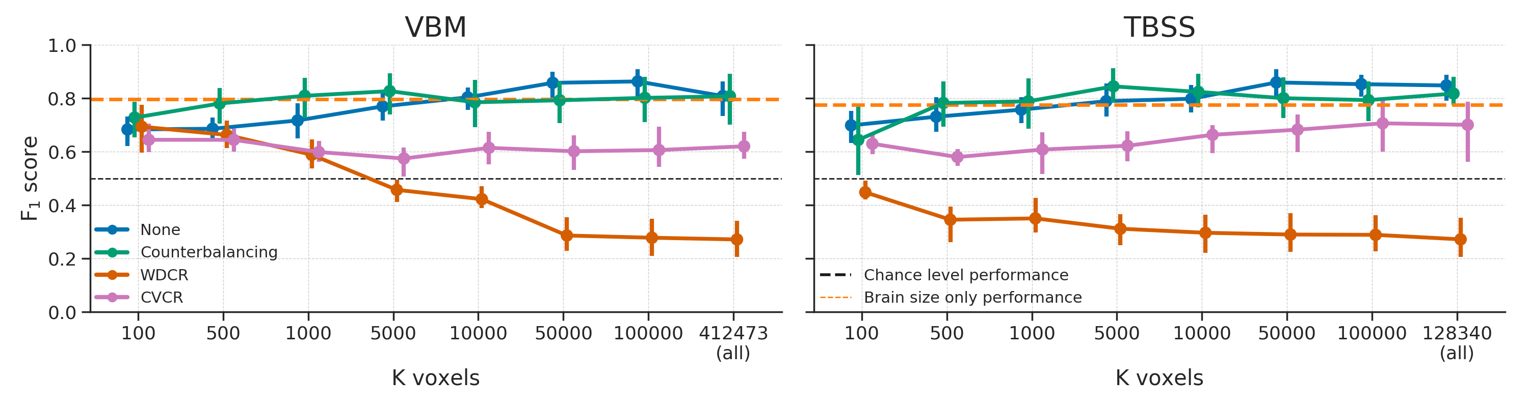
Figure 3.16: An overview of the empirical results on the four different confound methods: None, post hoc counterbalancing, WDCR, and CVCR.

3.4 Discussion

Decoding analyses have become a popular alternative to univariate analyses of neuroimaging data. This analysis approach, however, inherently suffers from ambiguity in terms of which source of information is picked up by the decoder (Naselaris & Kay, 2015). Given that one is often interested in model interpretability rather than merely accurate prediction (Hebart & Baker, 2017), one should strive to control for alternative sources of information (i.e., other than the target of interest) that might drive decoding. Effectively controlling for these alternative sources of information, or confounds, helps in disambiguating decoding models. In this article, we reviewed and tested two generic, broadly applicable methods that aim to control for confounds in decoding analyses: post hoc counterbalancing and confound regression. Additionally, we proposed a third method that, unlike the other two methods, has shown to effectively control for confounds.

Both when applied to empirical and simulated data, we found that neither post hoc counterbalancing nor (whole-dataset) confound regression yielded plausible and unbiased model performance estimates. First, we found that post hoc counterbalancing leads to optimistic (i.e., positively biased) model performance estimates, which is a result of removing samples that are hard to classify or would be wrongly classified, during the subsampling process. Because this subsampling process is applied to the entire dataset at once (i.e., it is not cross-validated), it can be seen as a form of indirect circular analysis (Kriegeskorte et al., 2009), in which the data themselves are used to inform analysis decisions, which can lead to biased generalization estimates. Second, our initial evaluation of confound regression, which was applied on the entire dataset (“WDCR”), yielded pessimistic (i.e., negatively biased) and even significantly below chance model performance estimates. Extending previous research (Jamalabadi et al., 2016), we show that this negative bias occurs when the “signal” in the data (operationalized as the width of the feature-target correlation distribution) is lower than would be expected by chance, which we link to the sampling distribution of the Pearson correlation coefficient. Importantly, we show that WDCR systematically narrows the width of the correlation distribution — and thus leads to lower model performance — which is exacerbated by both higher correlations between target and confound, as well as by a larger number of features.

The negative bias observed in WDCR is caused by the fact that it is performed on the whole dataset at once, leading to statistical dependencies between subsequent train and test partitions. To overcome this negative bias, we propose to cross-validate the confound regression procedure (which we call “Cross-Validated Confound Regression”, CVCR). We show that this method yields plausible model performance in the empirical analyses (i.e., significantly above chance model performance) and nearly unbiased model performance in the simulations, for different datasets varying in the amount of features ($K$) and the strength of the confound ($r_{Cy}$). Moreover, initial supplementary simulations suggest that these results generalize to (simulated) fMRI data (Supplementary Figure B.1), seemingly demonstrating effective control of confounds across different degrees of autocorrelation (Supplementary Figure B.2). The method may show some negative bias in some scenarios due to the fact that, in the train set, CVCR will remove all variance associated with the confound (even variance spuriously correlated with the confound). However, this bias seems, at least in the simulated scenarios, very small. Overall, we believe that our results demonstrate that CVCR is a flexible and effective method to control for confounds in decoding analyses of neuroimaging data.

3.4.1 Relevance and consequences for previous and future research

3.4.1.1 A priori and post hoc counterbalancing

We believe our results have implications not only for post hoc counterbalancing, but a priori counterbalancing in observational designs in general. In both behavioral research (Wacholder et al., 1992) and neuroimaging research (Görgen et al., 2017), a priori counterbalancing (or case-control “matching”) is a common strategy to avoid effects of confounds. However, as we show in the current study, this may unintentionally remove samples that are harder to predict, especially when there is little shared variance between the confound and the other predictors (i.e., when there is low confound $R^2$). Because, conceptually, this represents a form of circular analysis, counterbalancing — regardless of whether it is applied a priori or post hoc — can yield biased model performance estimates. To some extent, the bias in the post hoc counterbalancing results should not come as a surprise: as noted in the Methods section, counterbalancing in observational research requires the researcher to choose a sample that is not representative of the population (see also Sedgwick, 2013). As a result, out-of-sample predictive performance drops significantly, in our case even to chance level.

Since post hoc counterbalancing does not show any positive bias in model performance when there is no signal at all (i.e., signal $R^2$), one could argue that any observed significant above chance effect, while positively biased in terms of effect magnitude, can be interpreted as evidence that there must be signal in the data in the first place. However, we argue against this interpretation for two reasons. First, any above chance predictive performance of models fitted after subsampling is not only positively biased, but also does not cross-validate to the rejected samples (see Figure 3.11). That is, the model picks up relations between features and target that are only present in the subsample, and not in the samples left out of the analysis. As a result, it is questionable whether (and if so, how) the model should be interpreted — after all, we assume that the rejected samples were drawn from the population of interest in a valid way. Second, any possible absence of above chance model performance after subsampling can neither be interpreted as evidence for an absence of a true effect, since the subsampling procedure necessarily leads to a (often substantial) power loss. It could still well be that in the original sample there was a true relation between features and target. Thus, interpretation of modelling efforts after subsampling is problematic in case of both presence and absence of above chance model performances.

3.4.1.2 Confound regression

In contrast to post hoc counterbalancing, confound regression in its uncross-validated form (i.e., WDCR) has been applied widely in the context of decoding analyses (Dubois et al., 2018; Kostro et al., 2014; Rao et al., 2017; Todd et al., 2013). Indeed, the first study that systematically investigated the effect of confounds in decoding analyses (Todd et al., 2013) used WDCR to account for the confounding effect of reaction times (RT) on decoding of rule representations and found that WDCR completely eliminated the predictive performance that was found without controlling for RT. This observation, however, can potentially be explained by the negative bias induced by WDCR. This possible explanation is corroborated by a follow-up study that similarly looked into RT confounding the decoding of rule representations (Woolgar et al., 2014), who did not use WDCR but accounted for RT confounding by including it as a covariate during the pattern estimation procedure (see Supplementary Materials for a tentative evaluation of this method), which in contrast to the study by Todd et al. yielded significant decoding performance. Moreover, while not specifically investigated here, we expect a similar negative bias to occur when a confound is removed from a continuous target variable using WDCR — which may offer an explanation for the null finding of Dubois et al. (2018), who fail to decode personality characteristics from resting-state fMRI.

3.4.1.3 Relevance to other analysis methods

While this article focuses on controlling for confounds in decoding analyses specifically, we believe that our findings may be relevant for analysis methods beyond decoding analyses as well. In fact, methods for controlling for confounds (or alternative sources of information) have previously been investigated and applied in another type of MVPA named “representational similarity analysis” (RSA; Kriegeskorte et al., 2008). In the context of RSA, the explained variance in the neural data is often partitioned into different (model-based) feature sets (i.e., sources of information), which allows one to draw conclusions about the unique influence of each source of information (see, e.g., Groen et al., 2018; Hebart et al., 2018; Ramakrishnan et al., 2014). Specifically, variance partitioning in RSA is done by removing the variance from the representational dissimilarity matrix (RDM) based on the feature set that needs to be controlled for. Notably, the variance of the RDMs that are not of interest can be removed from only the neural RDM (Hebart et al., 2018; Ramakrishnan et al., 2014) or both from the neural RDM and the RDM of interest (Groen et al., 2018). While the analysis context is different, the underlying technique is identical to confound regression as described and evaluated in this article. Importantly, the studies employing this variance partitioning technique (Groen et al., 2018; Hebart et al., 2018; Ramakrishnan et al., 2014) similarly report plausible model performances after confound regression (i.e., relatively lower but not below chance performance), corroborating our results with (cross-validated) confound regression. Note that the distinction between WDCR and CVCR in the context of most RSA studies (including the aforementioned studies) is largely irrelevant, as representational similarity analyses are not commonly cross-validated. However, recently, some have proposed to use cross-validated distance measures (such as the cross-validated Mahalanobis distance; Guggenmos et al., 2018; Walther et al., 2016) in RSA, which could suffer from negative bias when combined with (not cross-validated) variance partitioning similar to what we observed with WDCR in the context of decoding analyses.

We believe that especially our findings with regard to WDCR and CVCR may be relevant for any cross-validated analysis, regardless of the “direction” of analysis (encoding vs. decoding) and the dimensionality of the neural data (univariate vs. multivariate approaches). In general, our findings with respect to negative bias after WDCR were to be expected, as it introduces dependence between the train set and the test set which violates the crucial assumption of independence of any cross-validated analysis. While a violation of the independence assumption often leads to positive bias such as in “double dipping” (Kriegeskorte et al., 2009), we show here that it may also lead to negative bias. Either way, our findings reinforce the idea that data analysis operations should never be applied to the entire dataset before subjecting the data to a cross-validated analysis. Therefore, we believe that our findings with respect to WDCR and CVCR will generalize to any cross-validated analysis (such as cross-validated MANOVA, Allefeld & Haynes, 2014; or cross-validated encoding models, Naselaris et al., 2011), but future research is necessary to substantiate this claim.

3.4.1.4 Importance for gender decoding studies

The importance of proper confound control is moreover highlighted by the empirical question we address. Without any optimization of the prediction pipeline, we were able to predict gender with a model performance up to approximately 0.85 without confound control. This is in line with reports from various other studies (Del Giudice et al., 2016; Rosenblatt, 2016; Sepehrband et al., 2018). However, this predictive performance is driven by a mixture two sources of information: global and local differences in brain structure. With confound control, however, we show that predictive performance using only local differences lies around 0.6 for VBM data and 0.7 for TBSS data — a substantial drop in performance. Especially because the remaining predictive performance is lower than predictive performance using only brain size, we argue that the use of proper confound control may lead one to draw substantially different conclusions about the differences in brain structure between men and women. For the debate on gender dimorphism, it is thus extremely important to take global brain size into account in the context of decoding analyses (as has been similarly recommended for mass-univariate analyses; Barnes et al., 2010).

3.4.2 Choosing a confound model: linear vs. nonlinear models

In the present paper, we focused on the use of linear models for confound control. It is crucial to note that the efficacy of confound control depends on the suitability of the confound regression model employed. Removing variance associated with a confound using a linear model removes only the variance of data (features) that is linearly related to the confound. When a confound is nonlinearly related to the data, some variance associated with the confound can remain in the data after a linear confound model is used to regress out variance. It is possible that the decoding model subsequently applied still picks up this residual “confounded” variance. In other words, an unsuitable confound model may control for confounds imperfectly.

The exact relation between confound and (brain) data is hardly ever known a priori. However, it is possible to explore the nature of this relation using the data at hand. For example, a researcher can apply a cross-validated prediction pipeline to predict a feature (e.g., VBM voxel intensity) from the confound. The researcher can then test what type of model (linear or nonlinear) describes the relation between confound and data best. In the Supplementary Materials (section “Linear vs nonlinear confound models: predicting VBM and TBSS data based on brain size”), we provide an example of this approach. We used linear, quadratic, and cubic regression models to predict VBM and TBSS voxel intensity using brain size as feature. In the Supplementary Results, we show that linear models perform equally well as or better than polynomial models for the majority of voxels (Supplementary Figures B.7 and B.9). Further, for voxels where polynomials outperform linear models, the difference between model performances is minimal (Supplementary Figure B.8). Thus, in the empirical research question explored in this paper, a linear confound model seems to suit the data very well.

3.4.3 Practical recommendations

As indicated by the title of this article, we will now outline some practical recommendations for dealing with confounds in decoding analyses of neuroimaging data. First, one needs to obtain an accurate measurement of potential confounds (Westfall & Yarkoni, 2016). While we assumed the availability of such a measure in this article, this is not always trivial. In experimental settings, for example, reaction times can potentially be identified as a confound (Todd et al., 2013; Woolgar et al., 2014), but arguably, it is not reaction time but rather an unobserved variable related to reaction time (e.g., difficulty or attention) that confounds the analysis. In such scenarios, the best one can do is measure reaction time as a proxy, and be aware that any subsequent confound control method is limited by how well this proxy corresponds to the actual confound. Second, one needs to identify which variables actually confound a decoding analysis. To detect confounds, we recommend using the “same analysis approach” outlined by Görgen et al. (2017). In short, this method involves trying to predict the target variable using your confound(s) as predictive features (for example, when using only brain size to predict gender). In case of significant above chance decoding performance, and assuming the confounds are actually encoded in the neuroimaging data, the hypothesized confounds will most likely influence the actual decoding analysis. While in the current article we focused on simple univariate confounding effects (i.e., confounding by a single variable), the same analysis approach is not limited to detecting univariate confounds — it facilitates detecting multivariate (i.e., confounding by multiple variables) or interaction effects (i.e., confounding by interaction effects between variables) as well. For example, if one hypothesizes that the target variable is related to the interaction between confound $C_{1}$ and $C_{2}$ (i.e., $C_{1} \times C_{2}$), one can simply use the interaction term as the potential confound in the same analysis approach to evaluate the potential confounding influence.

Once the specific confound terms have been identified, we recommend regressing out the confound from the data in a cross-validated manner (i.e., using CVCR). Specifically, we recommend including confound regression as the first step in your decoding pipeline to avoid the effect of confounds on other operations in the pipeline (such as univariate feature selection; Chu et al., 2012). In this article, we used ordinary least squares (OLS) regression to remove the influence of confounds from the data, because a linear model describes the relation between brain size and VBM/TBSS voxel intensities well (see Supplementary Figures B.7-B.9). However, not only linear models can be used to remove variance associated with a confound from the data — it is possible to use nonlinear models (potentially with multiple confounds and interactions between them) if it is clear that the relation between confounds and neuroimaging features is nonlinear (see previous section for details on choosing a confound model). However, as a limitation to the presented results, we did not test whether CVCR also leads to (nearly) unbiased results when used with nonlinear models. We advise, therefore, in such cases, to first test in a simulation study whether CVCR provides an unbiased confound control method with nonlinear models before use with actual data.

3.5 Conclusion

In general, we believe that the contributions of the current study are twofold. First and foremost, it provides a systematic evaluation of widely applicable methods to control for confounds and shows that, of the methods investigated, only one (“cross-validated confound regression”) appears to yield plausible and almost unbiased results. The results from this evaluation hopefully prevents researchers from using post hoc counterbalancing and whole-dataset confound regression, which we show may introduce (unintended) biases. Moreover, we made all analyses and preprocessed data openly available (https://github.com/lukassnoek/MVCA) and provide a simple implementation for cross-validated confound regression that interfaces with the popular scikit-learn package in the Python programming language. Second, we believe that this study improves understanding of the elusive phenomenon of below chance accuracy (building on previous work by Jamalabadi et al., 2016). In general, we hope that this study helps researchers in gaining more insight into their decoding analyses by providing a method that disentangles the contributions of different sources of information that may be encoded in their data.

The terms “gender” and “sex” are both used in the relevant research literature. Here, we use the term gender because we refer to self-reported identity in the data described below.↩︎
Note that information related to global brain size persists when researchers analyze the structural MRI data in a common, normalized brain space, because spatial registration “squeezes” relatively large brains into a smaller template, increasing voxel statistics (e.g., gray matter density in VBM analyses), and vice versa (Douaud et al., 2007). This effect of global brain size similarly affects functional MRI analyses (Brodtmann et al., 2009).↩︎
However, if accurate prediction is the only goal in this scenario, we would argue that there are probably easier and less expensive methods than neuroimaging to predict a participant’s gender.↩︎
In the context of behavioral data, a priori counterbalancing is often called “matching” or a employing a “case-control design” (Cook, 2002)↩︎
Note that the counterbalancing process is the same for both traditional univariate (activation-based) studies and decoding studies, but the direction of analysis is reversed in univariate (e.g., gender → brain) and decoding studies (e.g., brain → gender). As such, in univariate studies the confound (e.g., brain size) is counterbalanced with respect to the predictor(s) (e.g., gender) while in decoding studies the confound (e.g., brain size) is counterbalanced with respect to the target (e.g., gender).↩︎
However, parameter estimates only reflect unique variance when ordinary, weighted, or generalized least squares is used to find the model parameters. Other (regularized) linear models, such as ridge regression or LASSO, are not guaranteed to yield parameters that explain unique proportions of variance.↩︎
Note that $X$ and $C$, here, refer to (usually HRF-convolved) predictors of the time series signal ($s$) for a single voxel. In the rest of the article, $X$ and $C$ refer to features that are defined across samples (not time).↩︎
Note that, technically, one could use the “Control for confounds during pattern estimation” method in electrophysiology as well, by first fitting a univariate model explaining the neuroimaging data ($X_{j}$ for $j = 1 \dots K$) as a function of both the target ($y$) and the confound ($C$) and subsequently only using the parameter estimates of the target-predictor ($\hat{\beta}_{x}$) as patterns in the subsequent decoding analysis.↩︎
Note that we did not discuss studies that implement a different confound regression procedure (e.g., Abdulkadir et al., 2014; Dukart et al., 2011), in which confound regression is only estimated on the samples from a single class of the target variable (e.g., in our gender decoding example, this would mean that confound regression models are only estimated on the data from male, or female, subjects). As this form of confound regression does not disambiguate the sources of information driving the decoder, it is not discussed further in this article.↩︎
For continuous confounds, it is practically impossible to achieve a correlation with the target of exactly zero, which is the reason we subsample until it is smaller than a prespecified threshold. For categorical confounds, however, a correlation between the confound and the target of exactly zero is possible (this amounts to equal proportions of levels of $c$ within each class of $y$; Görgen et al., 2017), even necessary, because it is impossible to find a (K-fold) cross-validation partitioning in which each split is counterbalanced w.r.t. the confound if the correlation in the entire dataset between the target and the confound is not zero.↩︎
We refer to a relatively high α as “strict”, here, because we use it here for the purpose of demonstrating no effect.↩︎
One could run the “random subsampling” procedure with more than 10,000 draws in order to reduce the aforementioned power loss; but in the extreme, this would result in the same optimal subsample that can be found much faster by targeted subsampling.↩︎
Note that plausible null data do not reflect a signal $R^2$ of 0, because this statistic is biased towards values larger than 0 (because it represents a squared number) when dealing with noisy data, hence our choice of signal $R^2 = 0.004$.↩︎

Symbol	Dims.	Description
\(N\)		Number of samples (usually subjects or trials)
\(K\)		Number of neuroimaging features (e.g., voxels or sensors)
\(P\)		Number of confound variables (e.g., age, reaction time, or brain size)
\(X_{ij}\)	\(N \times K\)	The neuroimaging patterns (often called the “data” in the current article), where the subescript \(i \in {1 \dots N}\) refers to the individual samples (rows), and the subscript \(j \in {1 \dots K}\) to individual features (columns)
\(y\)	\(N \times 1\)	The target variable (i.e., what is to be decoded)
\(C\)	\(N \times P\)	The confound variable(s)
\(\hat{\beta}\)	\(K + 1\)	The parameters estimated in a general linear model (GLM)
\(w\)	\(K + 1\)	The parameters estimated in a decoding model
\(r_{Cy}\)		Sample Pearson correlation coefficient between \(C\) and \(y\)
\(r_{y(X.C)}\)		Sample semipartial Pearson correlation coefficient between \(X\) and \(y\), controlled for \(C\)
\(p(r_{Cy})\)		\(p\)-value of sample Pearson correlation between \(C\) and \(y\)
Note: Format based on Diedrichsen and Kriegeskorte (2017). For the correlations (\(r\)), we assume that \(P = 1\) and thus that the correlations in the table reduce to a scalar.