Extra exercises#
Although the previous tutorials contained several exercises, it doesn’t hurt to practice some more! The following exercises will test your Python (and Pandas/Matplotlib) skills. Note that it does not contain any exercises on Numpy because this is not directly relevant to the Python/PsychoPy course.
Basic Python#
The following ToDos help you practice with basic Python syntax and operations.
Show code cell content
""" Implement the ToDo here. """
x = -3.5

### BEGIN SOLUTION
y = (x + 5) ** 3
### END SOLUTION
""" Tests the above ToDo. """
assert(y == 3.375)
print("Well done!")
Well done!
Show code cell content
""" Implement the ToDo here. """
my_list = ['a', 'b', 'c', 'd', 'e', 'f', 'g', 'h']

### BEGIN SOLUTION
my_list_index_odd = my_list[1::2]
### END SOLUTION
""" Tests the above ToDo. """
assert(my_list_index_odd == ['b', 'd', 'f', 'h'])
print("Well done!")
Well done!
Show code cell content
""" Implement the ToDo here. """
my_list2 = ['hello', 'dear', 'student', ',', 'good', 'luck', 'on', 'this', 'ToDo!']

### BEGIN SOLUTION
my_list_filtered = [s for s in my_list2 if len(s) > 4]
# or:
my_list_filtered = []
for s in my_list2:
    if len(s) > 4:
        my_list_filtered.append(s)
### END SOLUTION
my_list_filtered
['hello', 'student', 'ToDo!']
""" Tests the above ToDo. """
assert(my_list_filtered == ['hello', 'student', 'ToDo!'])
print("Well done!")
Well done!
Show code cell content
""" Implement the ToDo here. """
my_list3 = [1, 8, -4, 0, 5820, 6823591, 99, 87, 27, 2386, 1242, 1111, 582353]
### BEGIN SOLUTION
my_list_even = [v for v in my_list3 if v % 2 == 0]
# or:
my_list_even = []
for v in my_list3:
    if v % 2 == 0:
        my_list_even.append(v)
### END SOLUTION
""" Tests the above ToDo. """
assert(sorted(my_list_even) == [-4, 0, 8, 1242, 2386, 5820])
print("Well done!")
Well done!
Show code cell content
""" Implement the ToDo here. """
graded_per_day = [20, 10, 8, 12]

### BEGIN SOLUTION
percentage_per_day = [v / sum(graded_per_day) * 100 for v in graded_per_day]
### END SOLUTION
""" Tests the above ToDo. """
assert([float(p) for p in percentage_per_day] == [40.0, 20.0, 16.0, 24.0])
print("Well done!")
Well done!
Compute the covariance (a single float!) between the two lists (z1 and z2) below and store it in a variable with the name cov_z1z2. You may use the order of steps below:
Compute the mean of the two lists
Create two new lists in which each value has been subtracted with the list’s mean
Write a for-loop (or list comprehension) that multiplies each value in one list with the corresponding value in the other list (resulting in another list)
Sum the results from the previous step
Divide the result by the length of the list minus 1
Show code cell content
""" Implement the ToDo here. """
import random
z1 = [random.uniform(0, 1) for _ in range(20)]
z2 = [random.uniform(0, 1) for _ in range(20)]

### BEGIN SOLUTION
z1c = [v - (sum(z1) / len(z1)) for v in z1]
z2c = [v - (sum(z2) / len(z2)) for v in z2]
z1z2 = [z1c[i] * z2c[i] for i in range(len(z1c))]
cov_z1z2 = sum(z1z2) / (len(z1c) - 1)
### END SOLUTION
""" Tests the above ToDo. """
import numpy as np
assert(round(cov_z1z2, 3) == round(np.cov(z1, z2)[0, 1], 3))
print("Well done!")
Well done!
Matplotlib#
Two Matplotlib exercises (both relatively difficult).
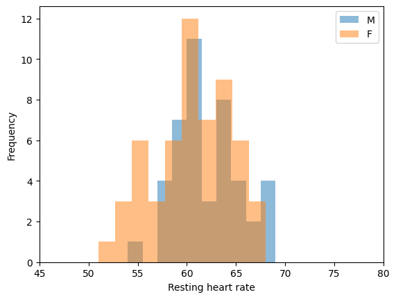
Show code cell content
""" Implement the ToDo here. """
np.random.seed(42)
rhr = np.random.normal(62, 4, size=500).astype(int).tolist()
gend = [np.random.choice(['M', 'F']) for _ in range(500)]

### BEGIN SOLUTION
import matplotlib.pyplot as plt
for g in ['M', 'F']:
    data = [rhr[i] for i in range(100) if gend[i] == g]
    plt.hist(data, alpha=0.5)

plt.legend(['M', 'F'])
plt.xticks([45, 50, 55, 60, 65, 70, 75, 80])
plt.ylabel('Frequency')
plt.xlabel('Resting heart rate')
#plt.savefig('rhr_by_gender.png')
plt.show()
### END SOLUTION
""" Tests the above ToDo. """
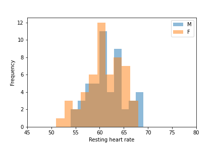
# Your plot should look like the one below!
from IPython.display import Image
Image('rhr_by_gender.png')
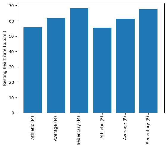
- People with a RHR < 58 ("athletic")
- People with a 58 ≤ RHR ≤ 65("average")
- People with a RHR > 65 ("sedentary")
Do this separately for men (“M”) and women (“F”), such that there are six bars (athletic/men, athletic/women, average/men, average/women, sedentary/men, sedentary/women).
Show code cell content
""" Implement the ToDo here. Requires quite a lot of code! """

### BEGIN SOLUTION
avs = []
for g in ['M', 'F']:
    dat = [rhr[i] for i in range(len(rhr)) if gend[i] == g]
    dat_ath = [val for val in dat if val < 58]
    avs.append(sum(dat_ath) / len(dat_ath))
    dat_ave = [val for val in dat if val >= 58 or val <= 65]
    avs.append(sum(dat_ave) / len(dat_ave))
    dat_sed = [val for val in dat if val > 65]
    avs.append(sum(dat_sed) / len(dat_sed))

labels = ['Athletic (M)', 'Average (M)', 'Sedentary (M)',
          'Athletic (F)', 'Average (F)', 'Sedentary (F)',
         ]
plt.bar(labels, avs)
plt.xticks(labels, rotation=90)
plt.ylabel('Resting heart rate (b.p.m.)')
plt.show()
### END SOLUTION
""" Tests the above ToDo. """
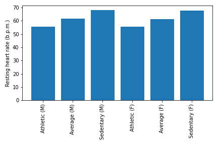
# Your plot should look like the one below!
from IPython.display import Image
Image('rhr_stratified.png')
Pandas#
Some Pandas exercises.
import random
import pandas as pd

n = 30
df = pd.DataFrame({
    'participant_id': ['sub-' + str(i).zfill(2) for i in range(1, n + 1)],
    'gender': [random.choice(['M', 'F']) for _ in range(n)],
    'condition': ['A', 'B', 'C'] * (n // 3),
    'prop_correct': np.random.uniform(0.4, 1, size=n),
    'mean_rt': np.random.normal(200, 20, n)
})
df.iloc[np.random.choice(range(n), size=2), -1] = np.nan
Show code cell content
""" Implement the ToDo here. """

### BEGIN SOLUTION
df_clean = df.dropna(axis=0)
### END SOLUTION
""" Tests the above ToDo. """
assert(df_clean.shape[0] == df.shape[0] - 2)
assert(df_clean.shape[1] == df.shape[1])

print("Well done.")
Well done.
Let’s delete the original df for now:
del df
Show code cell content
""" Implement the ToDo here. """

### BEGIN SOLUTION
idx = df_clean.loc[:, 'gender'] == 'M'
df_m = df_clean.loc[idx, :]
### END SOLUTION
""" Tests the above ToDo. """
assert(all(df_m.loc[:, 'gender'] == 'M'))
print("Well done!")
Well done!
Show code cell content
""" Implement the ToDo here. """

### BEGIN SOLUTION
idx = (df_clean.loc[:, 'prop_correct'] > 0.65) & (df_clean.loc[:, 'mean_rt'] < 200)
df_select = df_clean.loc[idx, :]
### END SOLUTION
""" Tests the above ToDo. """
assert(all(df_select.loc[:, 'mean_rt'] < 200))
assert(all(df_select.loc[:, 'prop_correct'] > 0.65))

print("Well done!")
Well done!
Show code cell content
""" Implement the ToDo here. """

### BEGIN SOLUTION
mu = df_clean.loc[:, 'prop_correct'].mean()
for idx in df_clean.index:
    if df_clean.loc[idx, 'prop_correct'] > mu:
        df_clean.loc[idx, 'status'] = 'above_average'
    else:
        df_clean.loc[idx, 'status'] = 'below_average'
### END SOLUTION
""" Tests the above ToDo. """
assert(all(df_clean.query("status == 'below_average'")['prop_correct'] < df_clean['prop_correct'].mean()))
assert(all(df_clean.query("status == 'above_average'")['prop_correct'] > df_clean['prop_correct'].mean()))
print("Well done!")
Well done!
Show code cell content
""" Implement the ToDo here. """
### BEGIN SOLUTION
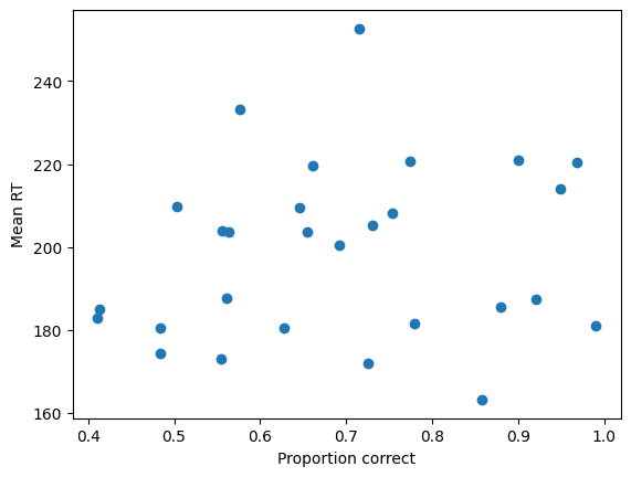
plt.scatter(df_clean.loc[:, 'prop_correct'], df_clean.loc[:, 'mean_rt'])
plt.xlabel('Proportion correct')
plt.ylabel('Mean RT')
plt.show()
### END SOLUTION
Note that, in real life, doing such “subgroup” analyses is probably a bad idea ;-)
Show code cell content
""" Implement the ToDo here. """
from scipy.stats import pearsonr

### BEGIN SOLUTION
corrs_conditions = []
for group in ['A', 'B', 'C']:
    tmp = df_clean.loc[df_clean.loc[:, 'condition'] == group, :]
    corr = pearsonr(tmp.loc[:, 'mean_rt'], tmp.loc[:, 'prop_correct'])[0]
    corrs_conditions.append(corr)
### END SOLUTION
""" Tests the above ToDo. Don't use this implementation ;-)"""
ans = df_clean.groupby('condition')[['mean_rt', 'prop_correct']].corr().iloc[1::2, 0].tolist()
np.testing.assert_array_almost_equal(ans, corrs_conditions, decimal=4)
print("Well done!")
Well done!