The Jupyter ecosystem#
In this course, we will use several tools from project Jupyter [Kluyver et al., 2016]. This project includes several nifty tools to make programming a little easier!
JupyterHub#
One tool that we use in this course is “JupyterHub”. This piece of software allows you to easily create a preconfigured Python environment on an external server — no need to install Python on your own computer anymore! You just go to the website/public IP associated with the external server and you can start programming! We run JupyterHub on our own server at the University of Amsterdam, which Research Master students can use for this course. Others may use the aforementioned tool “Binder” to create a JupyterHub instance themselves, which can be used for this course as well!
Jupyter interfaces: classic vs. JupyterLab#
The Jupyter environment offers two interfaces: the classic interface and the more extensive JupyterLab interface. On our own JupyterHub instance, we enabled the classic interface by default, because the grading software we use only works with this interface. On Binder, the classic notebook is the default interface, as well.
Note
Both the classic interface and the JupyterLab interface are shipped with the Anaconda distribution, so no need to install them manually! If you, for whatever reason, do need to install them, you can do so using pip:
pip install {package-name}
Replace {package-name} with jupyter to install the classic notebook interface and with jupyterlab to (additionally) install the JupyterLab interface.
Also, while on JupyterHub (including Binder) the Jupyter environment is always running, on your own computer you need to start it manually by running the following command in your terminal (or CMD prompt/Anaconda prompt/Powershell on Windows):
jupyter notebook
which opens the classic interface. To open the JupyterLab interface, run the following:
jupyter lab
These command will open a (new) tab in your default browser with the Jupyter interface. Note that, to stop the interface on your own computer, you need to stop the terminal process you started by typing Control (or Command) + C (or simply closing the terminal).
Both interfaces allow you to write, edit, and run code. Note that this is not limited to Python code! By installing different kernels, you can run programs written in many different programming languages, including R, Julia, and even Matlab. In fact, the name “Jupyter” is a reference to the three core programming languages supported by Jupyter: Julia, Python, and R.
In the Jupyter environment, code can be written and executed in different ways, which can be roughly divided into “script-based” and “interactive” approaches. In the script-based approach, you write your Python code in plain-text Python files (i.e., files with the extension .py) and run them, as a whole, in the terminal. In the interactive approach, you can write and run code interactively in either a Python console (or shell) or in a Jupyter notebook. The Jupyter notebook is the most common format for interactive computing and we will use it heavily in week 1 of this course. The next sections explains Jupyter Notebooks in more detail.
For now, if you want to quickly explore the Jupyter environment, you can click one of the two buttons below, which will access JupyterHub instance (with a classic interface) that includes the course materials. The UvA JupyterHub (orange button) is only accessible to Research Master Students enrolled in the “Programming for Psychology” course; instructions on how to log in onto the UvA JupyterHub can be found on Canvas. The Binder JupyterHub (blue button) can be used by anyone.
Note that, instead of using the classic interface, you can launch the JupyterLab interface by replacing the /tree snippet in the URL to /lab. To change it back to the classic interface again, click on Help → Launch Classic Notebook or change the /lab snippet back to /tree in the URL.
Jupyter Notebooks#
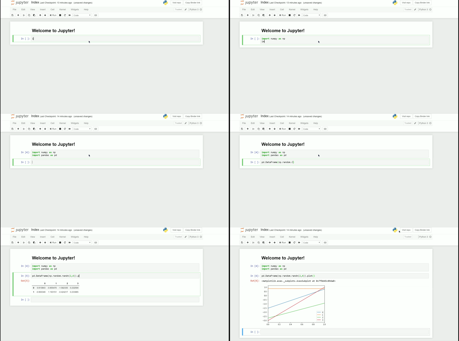
As mentioned, we use “Jupyter Notebooks” a lot in this course. Jupyter notebooks are very similar to R Markdown files. Like R Markdown files, you can mix text, code, plots, and mathematical formulas within a single document (see gif below).
 Gif from Cornellius Yudha Wijaya on towardsdatascience.com
Most of our tutorials are actually written in Jupyter notebooks. These notebooks are great for “interactive programming”, in which it is easy to experiment, try out, and troubleshoot your code. Because this mode of programming is great for teaching, we will use Jupyter notebooks a lot in week 1. Interactive programing is not, however, the only way in which you use Python. In fact, a lot of people use Python in a non-interactive way by writing scripts. In this “script mode” (for lack of a better term), writing the code and running the code are done separately. The code interface of PsychoPy (discussed in week 2), for example, cannot be used interactively and only supports “script mode”. We will dicuss both modes in this course.
If you want to check out Jupyter notebooks already, open a Jupyter interface (using Binder, the UvA JupyterHub, or on your own computer) and, in the upper right corner, click on New → Python 3 (in the classic interface) or click on the Python 3 tile in the launcher tab (in the JupyterLab interface).
Now, you should be ready to start on the course materials from week 1.
